전체 글
★=이 있는것이 귀무가설★모평균의 양측검정★모평균 <= |X 상단측 검정★모평균 >= |X 하단측검정★기초통계학-[연습문제 01 -09]
1. 모표준편차가 5인 정규모집단에서 크기 36인 표본을 추출했더니 표본평균이 48.5였다. 유의수준 5%에서 두 가설 H_0: m = 50과 H_1 : m != 50을 검정하려고 한다.
1> 기각역을 구하라.
x = np.arange(-5,5 , .001)

fig = plt.figure(figsize=(15,8))
ax = sns.lineplot(x , stats.norm.pdf(x, loc=0 , scale =1)) #정의역 범위 , 평균 = 0 , 표준편차 =1 인 정규분포 플롯

trust = 95 #신뢰도
# MEANS_A = 48.5
# MEANS_B = 50
# MEANS = MEANS_A-MEANS_B
# std_a = 5
# std_b = 5
# n_a = 55
# n_b = 47
# STDS = round(math.sqrt(std_a**2/n_a + std_b**2/n_b),3)
MEANS = 48.5
STDS = 5
n = 36

ax.set_title('양측검정' ,fontsize = 18)


#==========================================귀무가설 기각과 채택 ====================================================
trust = 95 #신뢰도_유의수준

t_1  = round(scipy.stats.norm.ppf(1 - (1-(trust/100))/2) ,3 )


ax.fill_between(x, stats.norm.pdf(x, loc=0 , scale =1) , 0 , where = (x<=t_1) & (x>=-t_1) , facecolor = 'orange') # x값 , y값 , 0 , x<=0 인곳 , 색깔
area = scipy.stats.norm.cdf(t_1) - scipy.stats.norm.cdf(-t_1)
ax.fill_between(x, stats.norm.pdf(x, loc=0 , scale =1) , 0 , where = (x>=t_1) | (x<=-t_1) , facecolor = 'red')
plt.annotate('' , xy=(0, .2), xytext=(2 , .2)  , arrowprops = dict(facecolor = 'black'))
ax.text(2 , .2, r'$H_{0}$의 채택역' +f'\nP({-t_1}<=Z<={t_1}) : {round(area,4)}',fontsize=15)

annotate_len = stats.norm.pdf(t_1, loc=0 , scale =1) /2
ax.vlines(x= t_1, ymin= 0 , ymax= stats.norm.pdf(t_1, loc=0 , scale =1) , color = 'green' , linestyle ='solid' , label ='{}'.format(2))
ax.vlines(x= -t_1, ymin= 0 , ymax= stats.norm.pdf(-t_1, loc=0 , scale =1) , color = 'green' , linestyle ='solid' , label ='{}'.format(2))

area = round((1-area)/2 ,3)
ax.text(1 + t_1 , annotate_len+0.02 , r'$z_{\alpha/2} = $' + f'{t_1}\n' + r'$H_{0}$의 기각역' + f'\n'+ r'$\alpha/2 = {%.3f}$' % area,fontsize=15)
ax.text(-2.5 -t_1 , annotate_len+0.02 , r'$z_{\alpha/2} = $' + f'{-t_1}\n' + r'$H_{0}$의 기각역' + f'\n'+ r'$\alpha/2 = {%.3f}$' % area,fontsize=15)


plt.annotate('' , xy=(t_1, annotate_len), xytext=(t_1+ 1 , annotate_len+0.02)  , arrowprops = dict(facecolor = 'black'))
plt.annotate('' , xy=(-t_1, annotate_len), xytext=(-1-t_1 , annotate_len+0.02)  , arrowprops = dict(facecolor = 'black'))


# ax.text(-5.5 , .25, f'신뢰구간 모평균에 대한 {trust}% : \n' + r'$\left( \overline{x}-\overline{y}\right)$' +f'-{t_1}' + r'$\sqrt{\dfrac{\sigma_{1}^{2}}{n}+\dfrac{\sigma_{2} ^{2}}{m}}$' +' , '+ r'$\left( \overline{x}-\overline{y}\right)$' +f'+ {t_1}' + r'$\sqrt{\dfrac{\sigma_{1}^{2}}{n}+\dfrac{\sigma_{2} ^{2}}{m}}$',fontsize=15)

ax.text(-5.5 , .15, f'신뢰구간 모평균에 대한 {trust}% : \n' + r'$\overline{X}$' +f'-{t_1}' + r'$\dfrac{\sigma}{\sqrt{n}},\overline{X}$' + f'+{t_1}' + r'$\dfrac{\sigma}{\sqrt{n}}$ ' ,fontsize=15)
ax.text(-5.5 , .25,  r'신뢰구간 L = $2*{%.3f}\dfrac{\sigma}{\sqrt{n}} $' % t_1 ,fontsize=15)

ax.text(-5.5 , .3,  r'오차한계 = ${%.3f}\dfrac{\sigma}{\sqrt{n}} $' % t_1,fontsize=15)

ax.text(2 , .35,  r'$\overline{X}$ = ' + f'{MEANS}\n' + r'$\sigma = $' + f'{STDS}\n' + r'$\sqrt{n} = $' + f'{round(math.sqrt(n),3)}',fontsize=15)
# ax.text(2 , .35,  r'$\overline{X}_{1}$ = ' +f'{MEANS_A}'+   r' , $\overline{X}_{2}$ = ' +f'{MEANS_B}\n' + r'$\sigma_{1} = $' + f'{std_a}' + r', $\sigma_{2} = $' + f'{std_b}\n' + r'$\sqrt{n} = $' + f'{round(math.sqrt(n_a),3)}' + r', $\sqrt{m} = $' + f'{round(math.sqrt(n_b),3)}',fontsize=15)


#============================================표본평균의 정규분포화 =========================================================
z_1 = round((MEANS-50)/ math.sqrt(STDS**2/n) ,2)
# # z_2 = round((34.5 - 35) / math.sqrt(5.5**2 / 25) , 2)
# z_1 = round(scipy.stats.norm.ppf(1 - (1-(trust/100))/2) ,3 )
print(z_1)
ax.fill_between(x, stats.norm.pdf(x, loc=0 , scale =1) , 0 , where = (x>=-z_1) | (x<=z_1) , facecolor = 'skyblue') # x값 , y값 , 0 , x<=0 인곳 , 색깔
ax.fill_between(x, stats.norm.pdf(x, loc=0 , scale =1) , 0 , where = (x>=t_1) | (x<=-t_1) , facecolor = 'red') # x값 , y값 , 0 , x<=0 인곳 , 색깔
area = scipy.stats.norm.cdf(z_1) + 1- scipy.stats.norm.cdf(-z_1)


ax.vlines(x= z_1, ymin= 0 , ymax= stats.norm.pdf(z_1, loc=0 , scale =1) , color = 'black' , linestyle ='solid' , label ='{}'.format(2))
ax.vlines(x= -z_1, ymin= 0 , ymax= stats.norm.pdf(-z_1, loc=0 , scale =1) , color = 'black' , linestyle ='solid' , label ='{}'.format(2))

annotate_len = stats.norm.pdf(z_1, loc=0 , scale =1) /2
plt.annotate('' , xy=(-z_1, annotate_len), xytext=(-z_1- 1 , annotate_len)  , arrowprops = dict(facecolor = 'black'))
plt.annotate('' , xy=(z_1, annotate_len), xytext=(1+z_1 , annotate_len)  , arrowprops = dict(facecolor = 'black'))
ax.text(-1.5 , annotate_len+0.01 , f'P-VALUE: \n  P(Z<={z_1}) + P(Z>={-z_1})  = {round(area,4)}',fontsize=15)


b= 'N(0,1)'

plt.legend([b] , fontsize = 15 , loc='upper left')
https://knowallworld.tistory.com/302
★모분산을 모를땐 t-분포!★stats.norm.cdf()★모분산을 알때/모를때 표본평균의 표본분포★일표본
1. 표본평균의 표본분포(모분산을 아는 경우) ==> 표본평균에 대한 표본분포는 정규분포를 따른다. EX-01) 모평균 100 , 모분산 9인 정규모집단으로부터 크기 25인 표본을 임의로 추출 1> 표본평균 |X
knowallworld.tistory.com

z_1 = round((MEANS-50)/ math.sqrt(STDS**2/n) ,2)
Z > 1.96 , Z<-1.96
2>검정통계량의 관찰값을 구하라.
z_0 = -1.8
3> P-VALUE 값 구하기
P-VALUE : 0.0719
4> 검정통계량의 관찰값을 이용하여 귀무가설의 진위를 결정하라.
z_0 = -1.8은 Z<-1.96 , Z>1.96 안에 놓이지 않으므로 유의수준 5%에서 귀무가설 H_0 : m= 50을 채택한다. 즉 모평균이 50이라는 주장은 타당성이 있다.
5> p-value 값을 이용하여 귀무가설의 진위를 결정하라.
P-VALUE : 0.0719
alpha : 0.05
P-VALUE > alpha ==> 0.0719 > 0.05 ==> 귀무가설 H_0 : m = 50을 채택한다. 즉 모평균이 50이라는 주장은 타당성이 있다.
2. 모표준편차가 0.35인 정규모집단에서 크기 45인 표본을 추출했더니 표본평균이 3.2였다. 유의수준 5%에서 두 가설 H_0: m = 3.09 과 H_1 : m != 3.09 를 검정하려고 한다.
1>기각역을 구하라.
x = np.arange(-5,5 , .001)

fig = plt.figure(figsize=(15,8))
ax = sns.lineplot(x , stats.norm.pdf(x, loc=0 , scale =1)) #정의역 범위 , 평균 = 0 , 표준편차 =1 인 정규분포 플롯

trust = 95 #신뢰도
# MEANS_A = 48.5
# MEANS_B = 50
# MEANS = MEANS_A-MEANS_B
# std_a = 5
# std_b = 5
# n_a = 55
# n_b = 47
# STDS = round(math.sqrt(std_a**2/n_a + std_b**2/n_b),3)
MEANS = 3.2
STDS = 0.35
n = 45

ax.set_title('양측검정' ,fontsize = 18)


#==========================================귀무가설 기각과 채택 ====================================================
trust = 95 #신뢰도_유의수준

t_1  = round(scipy.stats.norm.ppf(1 - (1-(trust/100))/2) ,3 )


ax.fill_between(x, stats.norm.pdf(x, loc=0 , scale =1) , 0 , where = (x<=t_1) & (x>=-t_1) , facecolor = 'orange') # x값 , y값 , 0 , x<=0 인곳 , 색깔
area = scipy.stats.norm.cdf(t_1) - scipy.stats.norm.cdf(-t_1)
ax.fill_between(x, stats.norm.pdf(x, loc=0 , scale =1) , 0 , where = (x>=t_1) | (x<=-t_1) , facecolor = 'red')
plt.annotate('' , xy=(0, .2), xytext=(2 , .2)  , arrowprops = dict(facecolor = 'black'))
ax.text(2 , .2, r'$H_{0}$의 채택역' +f'\nP({-t_1}<=Z<={t_1}) : {round(area,4)}',fontsize=15)

annotate_len = stats.norm.pdf(t_1, loc=0 , scale =1) /2
ax.vlines(x= t_1, ymin= 0 , ymax= stats.norm.pdf(t_1, loc=0 , scale =1) , color = 'green' , linestyle ='solid' , label ='{}'.format(2))
ax.vlines(x= -t_1, ymin= 0 , ymax= stats.norm.pdf(-t_1, loc=0 , scale =1) , color = 'green' , linestyle ='solid' , label ='{}'.format(2))

area = round((1-area)/2 ,3)
ax.text(1 + t_1 , annotate_len+0.02 , r'$z_{\alpha/2} = $' + f'{t_1}\n' + r'$H_{0}$의 기각역' + f'\n'+ r'$\alpha/2 = {%.3f}$' % area,fontsize=15)
ax.text(-2.5 -t_1 , annotate_len+0.02 , r'$z_{\alpha/2} = $' + f'{-t_1}\n' + r'$H_{0}$의 기각역' + f'\n'+ r'$\alpha/2 = {%.3f}$' % area,fontsize=15)


plt.annotate('' , xy=(t_1, annotate_len), xytext=(t_1+ 1 , annotate_len+0.02)  , arrowprops = dict(facecolor = 'black'))
plt.annotate('' , xy=(-t_1, annotate_len), xytext=(-1-t_1 , annotate_len+0.02)  , arrowprops = dict(facecolor = 'black'))


# ax.text(-5.5 , .25, f'신뢰구간 모평균에 대한 {trust}% : \n' + r'$\left( \overline{x}-\overline{y}\right)$' +f'-{t_1}' + r'$\sqrt{\dfrac{\sigma_{1}^{2}}{n}+\dfrac{\sigma_{2} ^{2}}{m}}$' +' , '+ r'$\left( \overline{x}-\overline{y}\right)$' +f'+ {t_1}' + r'$\sqrt{\dfrac{\sigma_{1}^{2}}{n}+\dfrac{\sigma_{2} ^{2}}{m}}$',fontsize=15)

ax.text(-5.5 , .15, f'신뢰구간 모평균에 대한 {trust}% : \n' + r'$\overline{X}$' +f'-{t_1}' + r'$\dfrac{\sigma}{\sqrt{n}},\overline{X}$' + f'+{t_1}' + r'$\dfrac{\sigma}{\sqrt{n}}$ ' ,fontsize=15)
ax.text(-5.5 , .25,  r'신뢰구간 L = $2*{%.3f}\dfrac{\sigma}{\sqrt{n}} $' % t_1 ,fontsize=15)

ax.text(-5.5 , .3,  r'오차한계 = ${%.3f}\dfrac{\sigma}{\sqrt{n}} $' % t_1,fontsize=15)

ax.text(2 , .35,  r'$\overline{X}$ = ' + f'{MEANS}\n' + r'$\sigma = $' + f'{STDS}\n' + r'$\sqrt{n} = $' + f'{round(math.sqrt(n),3)}',fontsize=15)
# ax.text(2 , .35,  r'$\overline{X}_{1}$ = ' +f'{MEANS_A}'+   r' , $\overline{X}_{2}$ = ' +f'{MEANS_B}\n' + r'$\sigma_{1} = $' + f'{std_a}' + r', $\sigma_{2} = $' + f'{std_b}\n' + r'$\sqrt{n} = $' + f'{round(math.sqrt(n_a),3)}' + r', $\sqrt{m} = $' + f'{round(math.sqrt(n_b),3)}',fontsize=15)


#============================================표본평균의 정규분포화 =========================================================
z_1 = round((MEANS-3.09)/ math.sqrt(STDS**2/n) ,2)
# # z_2 = round((34.5 - 35) / math.sqrt(5.5**2 / 25) , 2)
# z_1 = round(scipy.stats.norm.ppf(1 - (1-(trust/100))/2) ,3 )
print(z_1)
ax.fill_between(x, stats.norm.pdf(x, loc=0 , scale =1) , 0 , where = (x>=z_1) | (x<=-z_1) , facecolor = 'skyblue') # x값 , y값 , 0 , x<=0 인곳 , 색깔
ax.fill_between(x, stats.norm.pdf(x, loc=0 , scale =1) , 0 , where = (x>=t_1) | (x<=-t_1) , facecolor = 'red') # x값 , y값 , 0 , x<=0 인곳 , 색깔
area = scipy.stats.norm.cdf(-z_1) + 1- scipy.stats.norm.cdf(z_1)


ax.vlines(x= -z_1, ymin= 0 , ymax= stats.norm.pdf(-z_1, loc=0 , scale =1) , color = 'black' , linestyle ='solid' , label ='{}'.format(2))
ax.vlines(x= z_1, ymin= 0 , ymax= stats.norm.pdf(z_1, loc=0 , scale =1) , color = 'black' , linestyle ='solid' , label ='{}'.format(2))

annotate_len = stats.norm.pdf(z_1, loc=0 , scale =1) /2
plt.annotate('' , xy=(z_1, annotate_len), xytext=(z_1- 1 , annotate_len)  , arrowprops = dict(facecolor = 'black'))
plt.annotate('' , xy=(-z_1, annotate_len), xytext=(1-z_1 , annotate_len)  , arrowprops = dict(facecolor = 'black'))
ax.text(-1.5 , annotate_len+0.01 , f'P-VALUE: \n  P(Z<={-z_1}) + P(Z>={z_1})  = {round(area,4)}',fontsize=15)


b= 'N(0,1)'

plt.legend([b] , fontsize = 15 , loc='upper left')

Z > 1.96 , Z<-1.96
2>검정통계량의 관찰값을 구하라.
z_0 = 2.11
3> P-VALUE 값 구하기
P-VALUE : 0.0349.
4> 검정통계량의 관찰값을 이용하여 귀무가설의 진위를 결정하라.
z_0 = 2.11은 Z<-1.96 , Z>1.96 안에 놓이므로 유의수준 5%에서 귀무가설 H_0 : m= 3.09를 기각한다. 즉 모평균이 50이라는 주장은 타당성이 없다.
5> p-value 값을 이용하여 귀무가설의 진위를 결정하라.
P-VALUE : 0.0349
alpha : 0.05
P-VALUE< alpha ==> 0.0349 < 0.05 ==> 귀무가설 H_0 : m = 3.09를 기각한다. 즉 모평균이 3.09이라는 주장은 타당성이 없다.
3. 우리나라 직장인의 연간 평균 독서량이 15.5권 이상이라는 출판협회의 주장을 알아보기 위하여 50명의 직장인을 임의로 선정하여 독서량을 조사한 결과 연간 평균 14.2권 이었다. 그리고 과거 조사한 자료에 따르면 직장인의 연간 평균 독서량은 표준편차가 3.4권인 정규분포를 따르는 것으로 알려져 있다. 이 자료를 근거로 출판협회의 주장에 대하여 유의수준 1%에서 조사하라.
|X = 14.2
n = 50
s = 3.4
trust = 99
H_0 : m >= 15.5 ==> 하단측 검정
x = np.arange(-5,5 , .001)

fig = plt.figure(figsize=(15,8))
ax = sns.lineplot(x , stats.norm.pdf(x, loc=0 , scale =1)) #정의역 범위 , 평균 = 0 , 표준편차 =1 인 정규분포 플롯

trust = 95 #신뢰도
# MEANS_A = 48.5
# MEANS_B = 50
# MEANS = MEANS_A-MEANS_B
# std_a = 5
# std_b = 5
# n_a = 55
# n_b = 47
# STDS = round(math.sqrt(std_a**2/n_a + std_b**2/n_b),3)
MEANS = 14.2
STDS = 3.4
n = 50

ax.set_title('하단측검정' ,fontsize = 18)


#==========================================귀무가설 기각과 채택 ====================================================
trust = 99 #신뢰도_유의수준

t_1  = round(scipy.stats.norm.ppf(1 - (1-(trust/100))) ,3 )


ax.fill_between(x, stats.norm.pdf(x, loc=0 , scale =1) , 0 , where = (x>=-t_1)  , facecolor = 'orange') # x값 , y값 , 0 , x<=0 인곳 , 색깔
area = 1- scipy.stats.norm.cdf(-t_1)

plt.annotate('' , xy=(0, .2), xytext=(2 , .2)  , arrowprops = dict(facecolor = 'black'))
ax.text(2 , .2, r'$H_{0}$의 채택역' +f'\nP(Z>={-t_1}) : {round(area,4)}',fontsize=15)

annotate_len = stats.norm.pdf(t_1, loc=0 , scale =1) /2
ax.vlines(x= -t_1, ymin= 0 , ymax= stats.norm.pdf(-t_1, loc=0 , scale =1) , color = 'green' , linestyle ='solid' , label ='{}'.format(2))
# ax.vlines(x= -t_1, ymin= 0 , ymax= stats.norm.pdf(-t_1, loc=0 , scale =1) , color = 'green' , linestyle ='solid' , label ='{}'.format(2))

area = round((1-area) ,3)
# ax.text(1 + t_1 , annotate_len+0.02 , r'$z_{\alpha} = $' + f'{t_1}\n' + r'$H_{0}$의 기각역' + f'\n'+ r'$\alpha = {%.3f}$' % area,fontsize=15)
ax.text(-2.5 -t_1 , annotate_len+0.02 , r'$z_{\alpha/2} = $' + f'{-t_1}\n' + r'$H_{0}$의 기각역' + f'\n'+ r'$\alpha/2 = {%.3f}$' % area,fontsize=15)


# plt.annotate('' , xy=(t_1, annotate_len), xytext=(t_1+ 1 , annotate_len+0.02)  , arrowprops = dict(facecolor = 'black'))
plt.annotate('' , xy=(-t_1, annotate_len), xytext=(-1-t_1 , annotate_len+0.02)  , arrowprops = dict(facecolor = 'black'))


# ax.text(-5.5 , .25, f'신뢰구간 모평균에 대한 {trust}% : \n' + r'$\left( \overline{x}-\overline{y}\right)$' +f'-{t_1}' + r'$\sqrt{\dfrac{\sigma_{1}^{2}}{n}+\dfrac{\sigma_{2} ^{2}}{m}}$' +' , '+ r'$\left( \overline{x}-\overline{y}\right)$' +f'+ {t_1}' + r'$\sqrt{\dfrac{\sigma_{1}^{2}}{n}+\dfrac{\sigma_{2} ^{2}}{m}}$',fontsize=15)

ax.text(-5.5 , .15, f'신뢰구간 모평균에 대한 {trust}% : \n' + r'$\overline{X}$' +f'-{t_1}' + r'$\dfrac{\sigma}{\sqrt{n}},\overline{X}$' + f'+{t_1}' + r'$\dfrac{\sigma}{\sqrt{n}}$ ' ,fontsize=15)
ax.text(-5.5 , .25,  r'신뢰구간 L = $2*{%.3f}\dfrac{\sigma}{\sqrt{n}} $' % t_1 ,fontsize=15)

ax.text(-5.5 , .3,  r'오차한계 = ${%.3f}\dfrac{\sigma}{\sqrt{n}} $' % t_1,fontsize=15)

ax.text(2 , .35,  r'$\overline{X}$ = ' + f'{MEANS}\n' + r'$\sigma = $' + f'{STDS}\n' + r'$\sqrt{n} = $' + f'{round(math.sqrt(n),3)}',fontsize=15)
# ax.text(2 , .35,  r'$\overline{X}_{1}$ = ' +f'{MEANS_A}'+   r' , $\overline{X}_{2}$ = ' +f'{MEANS_B}\n' + r'$\sigma_{1} = $' + f'{std_a}' + r', $\sigma_{2} = $' + f'{std_b}\n' + r'$\sqrt{n} = $' + f'{round(math.sqrt(n_a),3)}' + r', $\sqrt{m} = $' + f'{round(math.sqrt(n_b),3)}',fontsize=15)


#============================================표본평균의 정규분포화 =========================================================
z_1 = round((MEANS-15.5)/ math.sqrt(STDS**2/n) ,2)
# # z_2 = round((34.5 - 35) / math.sqrt(5.5**2 / 25) , 2)
# z_1 = round(scipy.stats.norm.ppf(1 - (1-(trust/100))/2) ,3 )
print(z_1)
#
# z_1 = abs(z_1)
ax.fill_between(x, stats.norm.pdf(x, loc=0 , scale =1) , 0 , where = (x<=z_1) , facecolor = 'skyblue') # x값 , y값 , 0 , x<=0 인곳 , 색깔
ax.fill_between(x, stats.norm.pdf(x, loc=0 , scale =1) , 0 , where = (x<=-t_1) , facecolor = 'red') # x값 , y값 , 0 , x<=0 인곳 , 색깔
area =  scipy.stats.norm.cdf(z_1)


# ax.vlines(x= -z_1, ymin= 0 , ymax= stats.norm.pdf(-z_1, loc=0 , scale =1) , color = 'black' , linestyle ='solid' , label ='{}'.format(2))
ax.vlines(x= z_1, ymin= 0 , ymax= stats.norm.pdf(z_1, loc=0 , scale =1) , color = 'black' , linestyle ='solid' , label ='{}'.format(2))

annotate_len = stats.norm.pdf(z_1, loc=0 , scale =1) /2
plt.annotate('' , xy=(z_1, annotate_len), xytext=( -3 - z_1 , annotate_len)  , arrowprops = dict(facecolor = 'black'))
# plt.annotate('' , xy=(-z_1, annotate_len), xytext=(1-z_1 , annotate_len)  , arrowprops = dict(facecolor = 'black'))
ax.text(-1.5 , annotate_len+0.01 , f'P-VALUE: \n  P( P(Z<={z_1})  = {round(area,4)}',fontsize=15)


b= 'N(0,1)'

plt.legend([b] , fontsize = 15 , loc='upper left')
p-value : 0.0035
alpha : 0.010
p-value < alpha ==> 0.0035 < 0.010 ==> 귀무가설 H_0 : m >= 15.5 은 기각 ==> 대립가설 H_0 : m< 15.5 채택한다.
4. 2주 동안 유럽 여행을 하는데 소요되는 평균 경비는 300만원을 초과한다고 한다. 이를 알아보기 위하여 어느 날 인천국제공항에서 유럽 여행을 다녀온 사람 70명을 임의로 선정하여 조사한 결과 여행 경비는 평균 310만원 이었다. 여행 경비는 표준편차가 25.6만 원인 정규분포를 따르는 것으로 알려져 있다. 이 자료를 근거로 평균 경비가 300만 원을 초과하는지 유의수준 5%에서 조사하라.
|X = 310
n = 70
s = 25.6
trust = 95
H_0 : m <= 300 ==> 상단측 검정( 부등호가 있는것 귀무가설 설정)
x = np.arange(-5,5 , .001)

fig = plt.figure(figsize=(15,8))
ax = sns.lineplot(x , stats.norm.pdf(x, loc=0 , scale =1)) #정의역 범위 , 평균 = 0 , 표준편차 =1 인 정규분포 플롯

trust = 95 #신뢰도
# MEANS_A = 48.5
# MEANS_B = 50
# MEANS = MEANS_A-MEANS_B
# std_a = 5
# std_b = 5
# n_a = 55
# n_b = 47
# STDS = round(math.sqrt(std_a**2/n_a + std_b**2/n_b),3)
MEANS = 310
STDS = 25.6
n = 70

ax.set_title('상단측검정' ,fontsize = 18)


#==========================================귀무가설 기각과 채택 ====================================================
trust = 95 #신뢰도_유의수준

t_1  = round(scipy.stats.norm.ppf(1 - (1-(trust/100))) ,3 )


ax.fill_between(x, stats.norm.pdf(x, loc=0 , scale =1) , 0 , where = (x<=t_1)  , facecolor = 'orange') # x값 , y값 , 0 , x<=0 인곳 , 색깔
area = scipy.stats.norm.cdf(t_1)

plt.annotate('' , xy=(0, .2), xytext=(2 , .2)  , arrowprops = dict(facecolor = 'black'))
ax.text(2 , .2, r'$H_{0}$의 채택역' +f'\nP(Z<={t_1}) : {round(area,4)}',fontsize=15)

annotate_len = stats.norm.pdf(t_1, loc=0 , scale =1) /2
ax.vlines(x= t_1, ymin= 0 , ymax= stats.norm.pdf(t_1, loc=0 , scale =1) , color = 'green' , linestyle ='solid' , label ='{}'.format(2))
# ax.vlines(x= -t_1, ymin= 0 , ymax= stats.norm.pdf(-t_1, loc=0 , scale =1) , color = 'green' , linestyle ='solid' , label ='{}'.format(2))

area = round((1-area) ,3)
ax.text(1 + t_1 , annotate_len+0.02 , r'$z_{\alpha} = $' + f'{t_1}\n' + r'$H_{0}$의 기각역' + f'\n'+ r'$\alpha = {%.3f}$' % area,fontsize=15)
# ax.text(-2.5 -t_1 , annotate_len+0.02 , r'$z_{\alpha/2} = $' + f'{-t_1}\n' + r'$H_{0}$의 기각역' + f'\n'+ r'$\alpha/2 = {%.3f}$' % area,fontsize=15)


plt.annotate('' , xy=(t_1, annotate_len), xytext=(t_1+ 1 , annotate_len+0.02)  , arrowprops = dict(facecolor = 'black'))
# plt.annotate('' , xy=(-t_1, annotate_len), xytext=(-1-t_1 , annotate_len+0.02)  , arrowprops = dict(facecolor = 'black'))


# ax.text(-5.5 , .25, f'신뢰구간 모평균에 대한 {trust}% : \n' + r'$\left( \overline{x}-\overline{y}\right)$' +f'-{t_1}' + r'$\sqrt{\dfrac{\sigma_{1}^{2}}{n}+\dfrac{\sigma_{2} ^{2}}{m}}$' +' , '+ r'$\left( \overline{x}-\overline{y}\right)$' +f'+ {t_1}' + r'$\sqrt{\dfrac{\sigma_{1}^{2}}{n}+\dfrac{\sigma_{2} ^{2}}{m}}$',fontsize=15)

ax.text(-5.5 , .15, f'신뢰구간 모평균에 대한 {trust}% : \n' + r'$\overline{X}$' +f'-{t_1}' + r'$\dfrac{\sigma}{\sqrt{n}},\overline{X}$' + f'+{t_1}' + r'$\dfrac{\sigma}{\sqrt{n}}$ ' ,fontsize=15)
ax.text(-5.5 , .25,  r'신뢰구간 L = $2*{%.3f}\dfrac{\sigma}{\sqrt{n}} $' % t_1 ,fontsize=15)

ax.text(-5.5 , .3,  r'오차한계 = ${%.3f}\dfrac{\sigma}{\sqrt{n}} $' % t_1,fontsize=15)

ax.text(2 , .35,  r'$\overline{X}$ = ' + f'{MEANS}\n' + r'$\sigma = $' + f'{STDS}\n' + r'$\sqrt{n} = $' + f'{round(math.sqrt(n),3)}',fontsize=15)
# ax.text(2 , .35,  r'$\overline{X}_{1}$ = ' +f'{MEANS_A}'+   r' , $\overline{X}_{2}$ = ' +f'{MEANS_B}\n' + r'$\sigma_{1} = $' + f'{std_a}' + r', $\sigma_{2} = $' + f'{std_b}\n' + r'$\sqrt{n} = $' + f'{round(math.sqrt(n_a),3)}' + r', $\sqrt{m} = $' + f'{round(math.sqrt(n_b),3)}',fontsize=15)


#============================================표본평균의 정규분포화 =========================================================
z_1 = round((MEANS-300)/ math.sqrt(STDS**2/n) ,2)
# # z_2 = round((34.5 - 35) / math.sqrt(5.5**2 / 25) , 2)
# z_1 = round(scipy.stats.norm.ppf(1 - (1-(trust/100))/2) ,3 )
print(z_1)

z_1 = abs(z_1)
ax.fill_between(x, stats.norm.pdf(x, loc=0 , scale =1) , 0 , where = (x>=z_1) , facecolor = 'skyblue') # x값 , y값 , 0 , x<=0 인곳 , 색깔
ax.fill_between(x, stats.norm.pdf(x, loc=0 , scale =1) , 0 , where = (x>=t_1) , facecolor = 'red') # x값 , y값 , 0 , x<=0 인곳 , 색깔
area =  1- scipy.stats.norm.cdf(z_1)


# ax.vlines(x= -z_1, ymin= 0 , ymax= stats.norm.pdf(-z_1, loc=0 , scale =1) , color = 'black' , linestyle ='solid' , label ='{}'.format(2))
ax.vlines(x= z_1, ymin= 0 , ymax= stats.norm.pdf(z_1, loc=0 , scale =1) , color = 'black' , linestyle ='solid' , label ='{}'.format(2))

annotate_len = stats.norm.pdf(z_1, loc=0 , scale =1) /2
plt.annotate('' , xy=(z_1, annotate_len), xytext=(z_1- 1 , annotate_len)  , arrowprops = dict(facecolor = 'black'))
# plt.annotate('' , xy=(-z_1, annotate_len), xytext=(1-z_1 , annotate_len)  , arrowprops = dict(facecolor = 'black'))
ax.text(-1.5 , annotate_len+0.01 , f'P-VALUE: \n  P(Z>={z_1})  = {round(area,4)}',fontsize=15)


b= 'N(0,1)'

plt.legend([b] , fontsize = 15 , loc='upper left')
p-value : 0.0005
alpha : 0.05
p-value < alpha ==> 0.0005 < 0.005 ==> 귀무가설 H_0 : m <= 300 은 기각 ==> 대립가설 H_0 : m> 300 채택한다.
5. 환경부는 휴대전화 케이스 코팅 중소기업들이 집중된 어느 지역에서 오염물질인 총탄화수소의 대기배출 농도가 평균 902 ppm이라고 한다. 이를 알아보기 위하여 이 지역의 중소기업 50곳의 총탄화수소 대기배출 농도를 조사한 결과, 평균 농도가 895ppm이고 표준편차가 25.1ppm이었다. 이 자료를 근거로 환경부의 주장에 대하여 유의수준 5%에서 조사하라.
|X = 895
n = 50
s = 25.1
trust = 95
H_0 : m == 902 ==> 양측검정
x = np.arange(-5,5 , .001)

fig = plt.figure(figsize=(15,8))
ax = sns.lineplot(x , stats.norm.pdf(x, loc=0 , scale =1)) #정의역 범위 , 평균 = 0 , 표준편차 =1 인 정규분포 플롯

trust = 95 #신뢰도
# MEANS_A = 48.5
# MEANS_B = 50
# MEANS = MEANS_A-MEANS_B
# std_a = 5
# std_b = 5
# n_a = 55
# n_b = 47
# STDS = round(math.sqrt(std_a**2/n_a + std_b**2/n_b),3)
MEANS = 895
STDS = 25.1
n = 50

ax.set_title('양측검정' ,fontsize = 18)


#==========================================귀무가설 기각과 채택 ====================================================
trust = 95 #신뢰도_유의수준

t_1  = round(scipy.stats.norm.ppf(1 - (1-(trust/100))/2) ,3 )


ax.fill_between(x, stats.norm.pdf(x, loc=0 , scale =1) , 0 , where = (x<=t_1) & (x>=-t_1) , facecolor = 'orange') # x값 , y값 , 0 , x<=0 인곳 , 색깔
area = scipy.stats.norm.cdf(t_1) - scipy.stats.norm.cdf(-t_1)
ax.fill_between(x, stats.norm.pdf(x, loc=0 , scale =1) , 0 , where = (x>=t_1) | (x<=-t_1) , facecolor = 'red')
plt.annotate('' , xy=(0, .2), xytext=(2 , .2)  , arrowprops = dict(facecolor = 'black'))
ax.text(2 , .2, r'$H_{0}$의 채택역' +f'\nP({-t_1}<=Z<={t_1}) : {round(area,4)}',fontsize=15)

annotate_len = stats.norm.pdf(t_1, loc=0 , scale =1) /2
ax.vlines(x= t_1, ymin= 0 , ymax= stats.norm.pdf(t_1, loc=0 , scale =1) , color = 'green' , linestyle ='solid' , label ='{}'.format(2))
ax.vlines(x= -t_1, ymin= 0 , ymax= stats.norm.pdf(-t_1, loc=0 , scale =1) , color = 'green' , linestyle ='solid' , label ='{}'.format(2))

area = round((1-area)/2 ,3)
ax.text(1 + t_1 , annotate_len+0.02 , r'$z_{\alpha/2} = $' + f'{t_1}\n' + r'$H_{0}$의 기각역' + f'\n'+ r'$\alpha/2 = {%.3f}$' % area,fontsize=15)
ax.text(-2.5 -t_1 , annotate_len+0.02 , r'$z_{\alpha/2} = $' + f'{-t_1}\n' + r'$H_{0}$의 기각역' + f'\n'+ r'$\alpha/2 = {%.3f}$' % area,fontsize=15)


plt.annotate('' , xy=(t_1, annotate_len), xytext=(t_1+ 1 , annotate_len+0.02)  , arrowprops = dict(facecolor = 'black'))
plt.annotate('' , xy=(-t_1, annotate_len), xytext=(-1-t_1 , annotate_len+0.02)  , arrowprops = dict(facecolor = 'black'))


# ax.text(-5.5 , .25, f'신뢰구간 모평균에 대한 {trust}% : \n' + r'$\left( \overline{x}-\overline{y}\right)$' +f'-{t_1}' + r'$\sqrt{\dfrac{\sigma_{1}^{2}}{n}+\dfrac{\sigma_{2} ^{2}}{m}}$' +' , '+ r'$\left( \overline{x}-\overline{y}\right)$' +f'+ {t_1}' + r'$\sqrt{\dfrac{\sigma_{1}^{2}}{n}+\dfrac{\sigma_{2} ^{2}}{m}}$',fontsize=15)

ax.text(-5.5 , .15, f'신뢰구간 모평균에 대한 {trust}% : \n' + r'$\overline{X}$' +f'-{t_1}' + r'$\dfrac{\sigma}{\sqrt{n}},\overline{X}$' + f'+{t_1}' + r'$\dfrac{\sigma}{\sqrt{n}}$ ' ,fontsize=15)
ax.text(-5.5 , .25,  r'신뢰구간 L = $2*{%.3f}\dfrac{\sigma}{\sqrt{n}} $' % t_1 ,fontsize=15)

ax.text(-5.5 , .3,  r'오차한계 = ${%.3f}\dfrac{\sigma}{\sqrt{n}} $' % t_1,fontsize=15)

ax.text(2 , .35,  r'$\overline{X}$ = ' + f'{MEANS}\n' + r'$\sigma = $' + f'{STDS}\n' + r'$\sqrt{n} = $' + f'{round(math.sqrt(n),3)}',fontsize=15)
# ax.text(2 , .35,  r'$\overline{X}_{1}$ = ' +f'{MEANS_A}'+   r' , $\overline{X}_{2}$ = ' +f'{MEANS_B}\n' + r'$\sigma_{1} = $' + f'{std_a}' + r', $\sigma_{2} = $' + f'{std_b}\n' + r'$\sqrt{n} = $' + f'{round(math.sqrt(n_a),3)}' + r', $\sqrt{m} = $' + f'{round(math.sqrt(n_b),3)}',fontsize=15)


#============================================표본평균의 정규분포화 =========================================================
z_1 = round((MEANS-902)/ math.sqrt(STDS**2/n) ,2)
# # z_2 = round((34.5 - 35) / math.sqrt(5.5**2 / 25) , 2)
# z_1 = round(scipy.stats.norm.ppf(1 - (1-(trust/100))/2) ,3 )
print(z_1)

z_1 = abs(z_1)
ax.fill_between(x, stats.norm.pdf(x, loc=0 , scale =1) , 0 , where = (x>=z_1) | (x<=-z_1) , facecolor = 'skyblue') # x값 , y값 , 0 , x<=0 인곳 , 색깔
ax.fill_between(x, stats.norm.pdf(x, loc=0 , scale =1) , 0 , where = (x>=t_1) | (x<=-t_1) , facecolor = 'red') # x값 , y값 , 0 , x<=0 인곳 , 색깔
area = scipy.stats.norm.cdf(-z_1) + 1- scipy.stats.norm.cdf(z_1)


ax.vlines(x= -z_1, ymin= 0 , ymax= stats.norm.pdf(-z_1, loc=0 , scale =1) , color = 'black' , linestyle ='solid' , label ='{}'.format(2))
ax.vlines(x= z_1, ymin= 0 , ymax= stats.norm.pdf(z_1, loc=0 , scale =1) , color = 'black' , linestyle ='solid' , label ='{}'.format(2))

annotate_len = stats.norm.pdf(z_1, loc=0 , scale =1) /2
plt.annotate('' , xy=(z_1, annotate_len), xytext=(z_1- 1 , annotate_len)  , arrowprops = dict(facecolor = 'black'))
plt.annotate('' , xy=(-z_1, annotate_len), xytext=(1-z_1 , annotate_len)  , arrowprops = dict(facecolor = 'black'))
ax.text(-1.5 , annotate_len+0.01 , f'P-VALUE: \n  P(Z<={-z_1}) + P(Z>={z_1})  = {round(area,4)}',fontsize=15)


b= 'N(0,1)'

plt.legend([b] , fontsize = 15 , loc='upper left')

p-value : 0.0488
alpha : 0.05
p-value < alpha ==> 0.0488 < 0.005 ==> 귀무가설 H_0 : m == 902 은 기각 ==> 대립가설 H_0 : m!= 902 채택한다.
'기초통계 > 대표본 가설검정' 카테고리의 다른 글
| ★표본비율의 정규분포화★모비율의 가설 검정★기초통계학-[연습문제 03 -11] (0) | 2023.01.16 |
|---|---|
| ★모평균의 가설 검정★기초통계학-[연습문제 02 -10] (1) | 2023.01.16 |
| ★합동표본비율★양측검정, 상단측검정, 하단측검정 구분하기★모비율 차의 검정★기초통계학-[통계적 가설검정 -08] (0) | 2023.01.15 |
| ★귀무가설 p<=0 하단측검정★귀무가설 p>=0 ==> 하단측검정★모비율의 검정★기초통계학-[통계적 가설검정 -07] (1) | 2023.01.15 |
| ★p-value값★검정통계량의 관찰값★모평균 차의 검정★기초통계학-[통계적 가설검정 -06] (0) | 2023.01.15 |
★합동표본비율★양측검정, 상단측검정, 하단측검정 구분하기★모비율 차의 검정★기초통계학-[통계적 가설검정 -08]
https://knowallworld.tistory.com/334
★모평균 , 모비율의 차에 대한 신뢰구간★모비율에 대한 오차한계 및 신뢰구간★기초통계학-[
16. 2014년에 초,중,고 학생 116000명을 대상으로 우리나라 통일에 대해 조사한 결과, '통일이 필요하다' 라는 응답이 53.5%로 나타났다. 통일이 필요하다고 생각하는 초.중.고 학생의 비율에 대한 95%
knowallworld.tistory.com
https://knowallworld.tistory.com/311
★표본비율의 차에 대한 표본분포★기초통계학-[모집단 분포와 표본분포 -12]
1. 두 표본비율의 차에 대한 표본분포 ==> 서로 독립이고 모비율이 각각 p_1 , p_2인 두 모집단에서 각각 크기 n,m인 표본 선정 ==> 표본의 크기가 충분히 크다면 https://knowallworld.tistory.com/301 ★모비율
knowallworld.tistory.com

1. 합동표본비율(pooled sample proportion)
==> 두 표본에 대한 성공의 횟수 x와 y에 대한 비율
^p = (x+y)/(n+m)
==> 크기 n과 m인 표본
EX-01) 어느 대기업에 대한 취업 성향을 알아보기 위하여 20대와 30대 그룹으로 나누어 각각 952명과 1043명을 대상으로 조사하였다. 그 결과 이 기업을 선호한 인원이 각각 627명과 651명 이었다. 이 기업에 대한 20대의 선호도가 30대보다 높은지 유의수준 5%에서 검정하라.
^p_1 = 627/952
^p_2 = 651/1043
n = 952
m = 1043
20대의 선호도를 p1
30대의 선호도를 p2
p1-p2 > 0를 대립가설로 설정하면 귀무가설은 H_0 : p_1 - p_2 <=0(20대의 선호도는 30대보다 낮다) 이고, 대립가설은 H_1 : p_1-p_2 >0 이다.
귀무가설 : p_1 - p_2 <=0(20대의 선호도는 30대보다 낮다.) ==> 상단측검정
대립가설 : p_1 - p_2 > 0
1> 기각역을 구하여 검정한다.
x = np.arange(-5,5 , .001)
fig = plt.figure(figsize=(15,8))
ax = sns.lineplot(x , stats.norm.pdf(x, loc=0 , scale =1)) #정의역 범위 , 평균 = 0 , 표준편차 =1 인 정규분포 플롯
# trust = 95 #신뢰도
p1 = 627/952
p2 = 651/1043
n = 952
m = 1043
ax.set_title('상단측검정' ,fontsize = 18)
#==========================================귀무가설 기각과 채택 ====================================================
trust = 95 #신뢰도_유의수준
t_1 = round(scipy.stats.norm.ppf(1-(1-(trust/100))) ,3 )
ax.fill_between(x, stats.norm.pdf(x, loc=0 , scale =1) , 0 , where = (x<=t_1) , facecolor = 'orange') # x값 , y값 , 0 , x<=0 인곳 , 색깔
area = scipy.stats.norm.cdf(t_1)
plt.annotate('' , xy=(0, .2), xytext=(2 , .2) , arrowprops = dict(facecolor = 'black'))
ax.text(2 , .2, r'$H_{0}$의 채택역' +f'\nP(Z<={t_1}) : {round(area,4)}',fontsize=15)
annotate_len = stats.norm.pdf(t_1, loc=0 , scale =1) /2
ax.vlines(x= t_1, ymin= 0 , ymax= stats.norm.pdf(t_1, loc=0 , scale =1) , color = 'green' , linestyle ='solid' , label ='{}'.format(2))
# ax.vlines(x= -t_1, ymin= 0 , ymax= stats.norm.pdf(-t_1, loc=0 , scale =1) , color = 'green' , linestyle ='solid' , label ='{}'.format(2))
area = round((1-area) ,3)
# ax.text(1 + t_1 , annotate_len+0.02 , r'$z_{\alpha} = $' + f'{t_1}\n' + r'$H_{0}$의 기각역' + f'\n'+ r'$\alpha = {%.3f}$' % area,fontsize=15)
ax.text(1.5 +t_1 , annotate_len+0.02 , r'$z_{\alpha} = $' + f'{t_1}\n' + r'$H_{0}$의 기각역' + f'\n'+ r'$\alpha = {%.3f}$' % area,fontsize=15)
# plt.annotate('' , xy=(t_1, annotate_len), xytext=(t_1+ 1 , annotate_len+0.02) , arrowprops = dict(facecolor = 'black'))
plt.annotate('' , xy=(t_1, annotate_len), xytext=(1+t_1 , annotate_len+0.02) , arrowprops = dict(facecolor = 'black'))
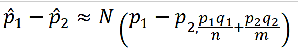
ax.text(-5.5 , .25, f'신뢰구간 모평균에 대한 {trust}% : \n' + r'$\left(\widehat{p}_{1} - \widehat{p}_{2}\right)$' +f'-{t_1}' + r'$\sqrt{\dfrac{\widehat{p}_{1}\widehat{q}_{1}}{n}+\dfrac{\widehat{p}_{2}\widehat{q}_{2}}{m}}$' +' , \n'+ r'$\left(\widehat{p}_{1} - \widehat{p}_{2}\right)$' +f'+ {t_1}' + r'$\sqrt{\dfrac{\widehat{p}_{1}\widehat{q}_{1}}{n}+\dfrac{\widehat{p}_{2}\widehat{q}_{2}}{m}}$',fontsize=15)
ax.text(-5.5 , .15, f'신뢰구간 모비율간 차에 대한 {trust}%의 합동표본비율 : \n' + r'$Z = \dfrac{\widehat{p}_1 - \widehat{p}_2}{ \sqrt{\widehat{p}\widehat{q} * (\dfrac{1}{n} + \dfrac{1}{m}}) }$',fontsize=15)
# ax.text(-5.5 , .25, f'귀무가설 : 남자(u_1)의 입원일수가 여자(u_2)의 입원일수 보다 작다.\n u_1 < u_2' , fontsize = 15)
ax.text(1 , .35, f' 신뢰구간 {trust}% 에 대한 오차 한계( ' +r'$e_{%d}) : $ '% trust + f'\n' + r'${%.3f}\sqrt{\dfrac{\widehat{p}_{1}\widehat{q}_{1}}{n}+\dfrac{\widehat{p}_{2}\widehat{q}_{2}}{m}}$ = '% t_1 + f'{round((t_1)*math.sqrt(p1*(1-p1)/n + p2*(1-p2)/m),3)} ' , fontsize= 15)
#============================================표본평균의 정규분포화 =========================================================
RATIO = round(p1 - p2,4)
SAMPLE_PROP = (627 + 651) / (952+1043)
STDS = math.sqrt( SAMPLE_PROP * (1-SAMPLE_PROP) * (1/n + 1/m))
# print(math.sqrt(SAMPLE_PROP * (1-SAMPLE_PROP) * (1/n + 1/m) ))
# print(RATIO)
# print(f'STDS :{STDS}' )
z_1 = round(RATIO/STDS , 4)
# z_1 =(9.075 - 7.114) / 1.6035
# # z_2 = round((34.5 - 35) / math.sqrt(5.5**2 / 25) , 2)
# z_1 = round(scipy.stats.norm.ppf(1 - (1-(trust/100))/2) ,3 )
print(z_1)
ax.fill_between(x, stats.norm.pdf(x, loc=0 , scale =1) , 0 , where = (x>=z_1) , facecolor = 'skyblue') # x값 , y값 , 0 , x<=0 인곳 , 색깔
ax.fill_between(x, stats.norm.pdf(x, loc=0 , scale =1) , 0 , where = (x>=t_1) , facecolor = 'red') # x값 , y값 , 0 , x<=0 인곳 , 색깔
area = 1- scipy.stats.norm.cdf(z_1)
ax.vlines(x= z_1, ymin= 0 , ymax= stats.norm.pdf(z_1, loc=0 , scale =1) , color = 'black' , linestyle ='solid' , label ='{}'.format(2))
# ax.vlines(x= -z_1, ymin= 0 , ymax= stats.norm.pdf(-z_1, loc=0 , scale =1) , color = 'black' , linestyle ='solid' , label ='{}'.format(2))
annotate_len = stats.norm.pdf(z_1, loc=0 , scale =1) /2
plt.annotate('' , xy=(z_1, annotate_len), xytext=(z_1- 1 , annotate_len) , arrowprops = dict(facecolor = 'black'))
# plt.annotate('' , xy=(-z_1, annotate_len), xytext=(1-z_1 , annotate_len) , arrowprops = dict(facecolor = 'black'))
ax.text(-1.5 , annotate_len+0.01 , f'P-VALUE: \n P(Z>={z_1}) = {round(area,4)}',fontsize=15)
b= 'N(0,1)'
plt.legend([b] , fontsize = 15 , loc='upper left')
#
# print( (9.075 - 7.114) / 1.6035)
2>p-값을 구하여 검정한다.
P-value = 0.0543
alpha = 0.05
귀무가설 : p_1 - p_2 <=0(20대의 선호도는 30대보다 낮다.) ==> 상단측검정
P-value > alpha ==> 0.0543 > 0.05 ==> 20대의 선호도가 30대보다 높다고 주장할 근거가 충분하지 않다.
EX-02) 어느 대학병원은 남자 1000명 중 56명 , 여자 1000명 중 37명이 심장 질환을 앓고 있다. 이를 기초로 하여 남녀의 심장 질환 발병 비율이 동일한지 유의수준 5%에서 검정하라.
남자의 심장 질환 발병 비율 : p1
여자의 심장 질환 발병 비율 : p2
귀무가설: p1 - p2 = 0 ==> 양측검정
대립가설 : p1 - p2 != 0
^p1 = 56/1000
^p2 = 37/1000
x = np.arange(-5,5 , .001)

fig = plt.figure(figsize=(15,8))
ax = sns.lineplot(x , stats.norm.pdf(x, loc=0 , scale =1)) #정의역 범위 , 평균 = 0 , 표준편차 =1 인 정규분포 플롯

# trust = 95 #신뢰도

ax.set_title('양측검정' ,fontsize = 18)
p1 = 56/1000
p2 = 37/1000

n = 1000
m = 1000

RATIO = round(p1 - p2,4)
print(RATIO)
SAMPLE_PROP = (56 + 37) / (1000+1000) #합동표본비율

STDS = math.sqrt( SAMPLE_PROP * (1-SAMPLE_PROP) * (1/n + 1/m))
print(STDS)


#==========================================귀무가설 기각과 채택 ====================================================
trust = 95 #신뢰도_유의수준

t_1  = round(scipy.stats.norm.ppf(1 - (1-(trust/100))) ,3 )


ax.fill_between(x, stats.norm.pdf(x, loc=0 , scale =1) , 0 , where = (x<=t_1) & (x>=-t_1) , facecolor = 'orange') # x값 , y값 , 0 , x<=0 인곳 , 색깔
area = 1- (1- scipy.stats.norm.cdf(t_1))

plt.annotate('' , xy=(0, .2), xytext=(2 , .2)  , arrowprops = dict(facecolor = 'black'))
ax.text(2 , .2, r'$H_{0}$의 채택역' +f'\nP({-t_1}<=Z<={t_1}) : {round(area,4)}',fontsize=15)

annotate_len = stats.norm.pdf(t_1, loc=0 , scale =1) /2
ax.vlines(x= t_1, ymin= 0 , ymax= stats.norm.pdf(t_1, loc=0 , scale =1) , color = 'green' , linestyle ='solid' , label ='{}'.format(2))
ax.vlines(x= -t_1, ymin= 0 , ymax= stats.norm.pdf(-t_1, loc=0 , scale =1) , color = 'green' , linestyle ='solid' , label ='{}'.format(2))
area = round((1-area)/2,6)
ax.text(1 + t_1 , annotate_len+0.02 , r'$z_{\alpha/2} = $' + f'{t_1}\n' + r'$H_{0}$의 기각역' + f'\n'+ r'$\alpha/2 = {%.4f}$' % area,fontsize=15)
ax.text(-2.5 -t_1 , annotate_len , r'$z_{\alpha/2} = $' + f'{-t_1}\n' + r'$H_{0}$의 기각역' + f'\n'+ r'$\alpha/2 = {%.3f}$' % area,fontsize=15)


plt.annotate('' , xy=(t_1, annotate_len-0.02), xytext=(t_1+ 1 , annotate_len)  , arrowprops = dict(facecolor = 'black'))
plt.annotate('' , xy=(-t_1, annotate_len-0.02), xytext=(-1-t_1 , annotate_len)  , arrowprops = dict(facecolor = 'black'))


ax.text(-5.5 , .25, f'신뢰구간 모평균에 대한 {trust}% : \n' + r'$\left(\widehat{p}_{1} - \widehat{p}_{2}\right)$' +f'-{t_1}' + r'$\sqrt{\dfrac{\widehat{p}_{1}\widehat{q}_{1}}{n}+\dfrac{\widehat{p}_{2}\widehat{q}_{2}}{m}}$' +' , \n'+ r'$\left(\widehat{p}_{1} - \widehat{p}_{2}\right)$' +f'+ {t_1}' + r'$\sqrt{\dfrac{\widehat{p}_{1}\widehat{q}_{1}}{n}+\dfrac{\widehat{p}_{2}\widehat{q}_{2}}{m}}$',fontsize=15)

ax.text(-5.5 , .15, f'신뢰구간 모비율간 차에 대한 {trust}%의 합동표본비율 : \n' + r'$Z = \dfrac{\widehat{p}_1 - \widehat{p}_2}{ \sqrt{\widehat{p}\widehat{q} * (\dfrac{1}{n} + \dfrac{1}{m}})  }$',fontsize=15)

ax.text(2 , .35 , r'합동표본비율의 $ \widehat{p} = \dfrac{x + y}{n + m}$' ,fontsize= 15)

# ax.text(-5.5 , .25, f'귀무가설 : 남자(u_1)의 입원일수가 여자(u_2)의 입원일수 보다 작다.\n u_1 < u_2'  , fontsize = 15)
# ax.text(1 , .35, f' 신뢰구간 {trust}% 에 대한 오차 한계( ' +r'$e_{%d}) : $ '% trust + f'\n' + r'${%.3f}\sqrt{\dfrac{\widehat{p}_{1}\widehat{q}_{1}}{n}+\dfrac{\widehat{p}_{2}\widehat{q}_{2}}{m}}$ = '% t_1 + f'{round((t_1)*math.sqrt(p1*(1-p1)/n + p2*(1-p2)/m),3)} ' , fontsize= 15)


# ax.text(-5.5 , .25,  r'신뢰구간 L = $2*{%.3f}\dfrac{\sigma}{\sqrt{n}} $' % t_1 ,fontsize=15)
#
# ax.text(-5.5 , .3,  r'오차한계 = ${%.3f}\dfrac{\sigma}{\sqrt{n}} $' % t_1,fontsize=15)


#============================================표본평균의 정규분포화 =========================================================

z_1 = round(RATIO/STDS  , 4)
print(z_1)
# # z_2 = round((34.5 - 35) / math.sqrt(5.5**2 / 25) , 2)
# z_1 = round(scipy.stats.norm.ppf(1 - (1-(trust/100))/2) ,3 )

ax.fill_between(x, stats.norm.pdf(x, loc=0 , scale =1) , 0 , where = (x>=z_1) | (x<=-z_1) , facecolor = 'skyblue') # x값 , y값 , 0 , x<=0 인곳 , 색깔
ax.fill_between(x, stats.norm.pdf(x, loc=0 , scale =1) , 0 , where = (x>=t_1) | (x<=-t_1) , facecolor = 'red') # x값 , y값 , 0 , x<=0 인곳 , 색깔
area =  scipy.stats.norm.cdf(-z_1) + 1 - (scipy.stats.norm.cdf(z_1))


ax.vlines(x= z_1, ymin= 0 , ymax= stats.norm.pdf(z_1, loc=0 , scale =1) , color = 'black' , linestyle ='solid' , label ='{}'.format(2))
ax.vlines(x= -z_1, ymin= 0 , ymax= stats.norm.pdf(-z_1, loc=0 , scale =1) , color = 'black' , linestyle ='solid' , label ='{}'.format(2))

annotate_len = stats.norm.pdf(z_1, loc=0 , scale =1) /2
plt.annotate('' , xy=(z_1, annotate_len), xytext=(-z_1/2 , annotate_len)  , arrowprops = dict(facecolor = 'black'))
plt.annotate('' , xy=(-z_1, annotate_len), xytext=(z_1/2 , annotate_len)  , arrowprops = dict(facecolor = 'black'))
ax.text(-1.5 , annotate_len+0.01 , f'P-value : \nP(Z<={-z_1}) + P(Z>={z_1}) \n = {round(area,4)}',fontsize=15)
# ax.text(0 , annotate_len+0.01 ,f'P(Z>={-z_1})',fontsize=15)


b= 'N(0,1)'

plt.legend([b] , fontsize = 15 , loc='upper left')
p-value : 0.0436
alpha = 0.05
p-value < alpha ==> 0.0436 < 0.05 ==> 귀무가설(남자의 심장발병 비율이 동일하다.) 는 기각
'기초통계 > 대표본 가설검정' 카테고리의 다른 글
| ★모평균의 가설 검정★기초통계학-[연습문제 02 -10] (1) | 2023.01.16 |
|---|---|
| ★=이 있는것이 귀무가설★모평균의 양측검정★모평균 <= |X 상단측 검정★모평균 >= |X 하단측검정★기초통계학-[연습문제 01 -09] (2) | 2023.01.16 |
| ★귀무가설 p<=0 하단측검정★귀무가설 p>=0 ==> 하단측검정★모비율의 검정★기초통계학-[통계적 가설검정 -07] (1) | 2023.01.15 |
| ★p-value값★검정통계량의 관찰값★모평균 차의 검정★기초통계학-[통계적 가설검정 -06] (0) | 2023.01.15 |
| ★p-value값★검정통계량의 관찰값★모평균에 대한 상단측 검정★기초통계학-[통계적 가설검정 -05] (0) | 2023.01.13 |
★귀무가설 p<=0 하단측검정★귀무가설 p>=0 ==> 하단측검정★모비율의 검정★기초통계학-[통계적 가설검정 -07]
EX-01) 대형마트 A는 고객의 이용률이 다른 마트들 보다 높은 45%라고 협력업체에 홍보하였다. 이러한 사실의 진위를 알아보기 위하여 협력 업체가 주민 1500명을 대상으로 조사한 결과, 642명이 A마트를 주로 이용한다고 답하였다.
https://knowallworld.tistory.com/327
★모비율의 신뢰구간★기초통계학-[대표본 추정 -04]
1. 모비율의 신뢰구간 https://knowallworld.tistory.com/306 이항분포에 따른 정규분포의 표준정규분포화★표본비율의 표본분포★기초통계학-[모집단 분포 1.표본비율의 표본분포 EX) 이항 확률변수의 실
knowallworld.tistory.com

1> A 마트의 주장을 유의수준 5%에서 검정하라.
귀무가설 : A이용률 - 타 이용률 = 0.45
n = 1500
^p = 642/1500
x = np.arange(-5,5 , .001)

fig = plt.figure(figsize=(15,8))
ax = sns.lineplot(x , stats.norm.pdf(x, loc=0 , scale =1)) #정의역 범위 , 평균 = 0 , 표준편차 =1 인 정규분포 플롯

# trust = 95 #신뢰도

ax.set_title('양측검정' ,fontsize = 18)
RATIO = round(642/1500 , 4)
n = 1500
MEANS = 0.45
STDS = round(math.sqrt((MEANS * (1-MEANS) / n)),4)
n = 50

#==========================================귀무가설 기각과 채택 ====================================================
trust = 95 #신뢰도_유의수준

t_1  = round(scipy.stats.norm.ppf(1 - (1-(trust/100))/2) ,3 )


ax.fill_between(x, stats.norm.pdf(x, loc=0 , scale =1) , 0 , where = (x<=t_1) & (x>=-t_1) , facecolor = 'orange') # x값 , y값 , 0 , x<=0 인곳 , 색깔
area = scipy.stats.norm.cdf(-t_1)

plt.annotate('' , xy=(0, .2), xytext=(2 , .2)  , arrowprops = dict(facecolor = 'black'))
ax.text(2 , .2, r'$H_{0}$의 채택역' +f'\nP({-t_1}<=Z<={t_1}) : {round(area,4)}',fontsize=15)

annotate_len = stats.norm.pdf(t_1, loc=0 , scale =1) /2
ax.vlines(x= t_1, ymin= 0 , ymax= stats.norm.pdf(t_1, loc=0 , scale =1) , color = 'green' , linestyle ='solid' , label ='{}'.format(2))
ax.vlines(x= -t_1, ymin= 0 , ymax= stats.norm.pdf(-t_1, loc=0 , scale =1) , color = 'green' , linestyle ='solid' , label ='{}'.format(2))

ax.text(1 + t_1 , annotate_len+0.02 , r'$z_{\alpha/2} = $' + f'{t_1}\n' + r'$H_{0}$의 기각역' + f'\n'+ r'$\alpha/2 = {%.3f}$' % area,fontsize=15)
ax.text(-2.5 -t_1 , annotate_len+0.02 , r'$z_{\alpha/2} = $' + f'{-t_1}\n' + r'$H_{0}$의 기각역' + f'\n'+ r'$\alpha/2 = {%.3f}$' % area,fontsize=15)


plt.annotate('' , xy=(t_1, annotate_len-0.02), xytext=(t_1+ 1 , annotate_len)  , arrowprops = dict(facecolor = 'black'))
plt.annotate('' , xy=(-t_1, annotate_len-0.02), xytext=(-1-t_1 , annotate_len)  , arrowprops = dict(facecolor = 'black'))


ax.text(-5.5 , .15, f'신뢰구간 모평균에 대한 {trust}% : \n' + r'$\widehat{p}$' +f' + {t_1}' + r'$\sqrt{\dfrac{\widehat{p}\widehat{q}}{n}}$' +' , '+ r'$\widehat{p}$' +f' - {t_1}' + r'$\sqrt{\dfrac{\widehat{p}\widehat{q}}{n}}$',fontsize=15)


# ax.text(-5.5 , .25,  r'신뢰구간 L = $2*{%.3f}\dfrac{\sigma}{\sqrt{n}} $' % t_1 ,fontsize=15)
#
# ax.text(-5.5 , .3,  r'오차한계 = ${%.3f}\dfrac{\sigma}{\sqrt{n}} $' % t_1,fontsize=15)


#============================================표본평균의 정규분포화 =========================================================

z_1 = round((RATIO-MEANS)/STDS,4)
print(z_1)
# # z_2 = round((34.5 - 35) / math.sqrt(5.5**2 / 25) , 2)
# z_1 = round(scipy.stats.norm.ppf(1 - (1-(trust/100))/2) ,3 )

ax.fill_between(x, stats.norm.pdf(x, loc=0 , scale =1) , 0 , where = (x<=z_1) | (x>=-z_1) , facecolor = 'skyblue') # x값 , y값 , 0 , x<=0 인곳 , 색깔
ax.fill_between(x, stats.norm.pdf(x, loc=0 , scale =1) , 0 , where = (x>=t_1) | (x<=-t_1) , facecolor = 'red') # x값 , y값 , 0 , x<=0 인곳 , 색깔
area = scipy.stats.norm.cdf(-z_1) - scipy.stats.norm.cdf(z_1)


ax.vlines(x= z_1, ymin= 0 , ymax= stats.norm.pdf(z_1, loc=0 , scale =1) , color = 'black' , linestyle ='solid' , label ='{}'.format(2))
ax.vlines(x= -z_1, ymin= 0 , ymax= stats.norm.pdf(-z_1, loc=0 , scale =1) , color = 'black' , linestyle ='solid' , label ='{}'.format(2))

annotate_len = stats.norm.pdf(z_1, loc=0 , scale =1) /2
plt.annotate('' , xy=(z_1, annotate_len), xytext=(z_1+ 1 , annotate_len)  , arrowprops = dict(facecolor = 'black'))
plt.annotate('' , xy=(-z_1, annotate_len), xytext=(-1-z_1 , annotate_len)  , arrowprops = dict(facecolor = 'black'))
ax.text(-1.5 , annotate_len+0.01 , f'P-value : \nP(Z<={z_1}) + P(Z>={-z_1})  = {round(1-area,4)}',fontsize=15)
# ax.text(0 , annotate_len+0.01 ,f'P(Z>={-z_1})',fontsize=15)


ax.text(2 , .3,  r'$\sqrt{\widehat{p}\widehat{q}} = $' + f'{round(math.sqrt(RATIO * (1-RATIO)),3)}\n'  + r'$\sqrt{n} = $' + f'{round(math.sqrt(n),2)} \n p = {MEANS} n = {n} \n' + r'N(p , ' + r'$\dfrac{pq}{n}) = $' + f'N({MEANS} , {round(MEANS*(1-MEANS)/ n ,4)})',fontsize=15)

b= 'N(0,1)'

plt.legend([b] , fontsize = 15 , loc='upper left')
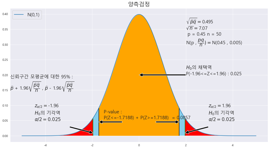
p-value : 0.0857
alpha : 0.5
p-value > alpha : 0.0857 > 0.5 ==> 귀무가설 p=0.45는 채택이된다.
2> p-값을 구하고 유의수준 10%에서 검정하라.
x = np.arange(-5,5 , .001)

fig = plt.figure(figsize=(15,8))
ax = sns.lineplot(x , stats.norm.pdf(x, loc=0 , scale =1)) #정의역 범위 , 평균 = 0 , 표준편차 =1 인 정규분포 플롯

# trust = 95 #신뢰도

ax.set_title('양측검정' ,fontsize = 18)
RATIO = round(642/1500 , 4)
n = 1500
MEANS = 0.45
STDS = round(math.sqrt((MEANS * (1-MEANS) / n)),4)
n = 50

#==========================================귀무가설 기각과 채택 ====================================================
trust = 90 #신뢰도_유의수준

t_1  = round(scipy.stats.norm.ppf(1 - (1-(trust/100))/2) ,3 )


ax.fill_between(x, stats.norm.pdf(x, loc=0 , scale =1) , 0 , where = (x<=t_1) & (x>=-t_1) , facecolor = 'orange') # x값 , y값 , 0 , x<=0 인곳 , 색깔
area = scipy.stats.norm.cdf(-t_1)

plt.annotate('' , xy=(0, .2), xytext=(2 , .2)  , arrowprops = dict(facecolor = 'black'))
ax.text(2 , .2, r'$H_{0}$의 채택역' +f'\nP({-t_1}<=Z<={t_1}) : {round(area,4)}',fontsize=15)

annotate_len = stats.norm.pdf(t_1, loc=0 , scale =1) /2
ax.vlines(x= t_1, ymin= 0 , ymax= stats.norm.pdf(t_1, loc=0 , scale =1) , color = 'green' , linestyle ='solid' , label ='{}'.format(2))
ax.vlines(x= -t_1, ymin= 0 , ymax= stats.norm.pdf(-t_1, loc=0 , scale =1) , color = 'green' , linestyle ='solid' , label ='{}'.format(2))

ax.text(1 + t_1 , annotate_len+0.02 , r'$z_{\alpha/2} = $' + f'{t_1}\n' + r'$H_{0}$의 기각역' + f'\n'+ r'$\alpha/2 = {%.3f}$' % area,fontsize=15)
ax.text(-2.5 -t_1 , annotate_len+0.02 , r'$z_{\alpha/2} = $' + f'{-t_1}\n' + r'$H_{0}$의 기각역' + f'\n'+ r'$\alpha/2 = {%.3f}$' % area,fontsize=15)


plt.annotate('' , xy=(t_1, annotate_len-0.02), xytext=(t_1+ 1 , annotate_len)  , arrowprops = dict(facecolor = 'black'))
plt.annotate('' , xy=(-t_1, annotate_len-0.02), xytext=(-1-t_1 , annotate_len)  , arrowprops = dict(facecolor = 'black'))


ax.text(-5.5 , .15, f'신뢰구간 모평균에 대한 {trust}% : \n' + r'$\widehat{p}$' +f' + {t_1}' + r'$\sqrt{\dfrac{\widehat{p}\widehat{q}}{n}}$' +' , '+ r'$\widehat{p}$' +f' - {t_1}' + r'$\sqrt{\dfrac{\widehat{p}\widehat{q}}{n}}$',fontsize=15)


# ax.text(-5.5 , .25,  r'신뢰구간 L = $2*{%.3f}\dfrac{\sigma}{\sqrt{n}} $' % t_1 ,fontsize=15)
#
# ax.text(-5.5 , .3,  r'오차한계 = ${%.3f}\dfrac{\sigma}{\sqrt{n}} $' % t_1,fontsize=15)


#============================================표본평균의 정규분포화 =========================================================

z_1 = round((RATIO-MEANS)/STDS,4)
print(z_1)
# # z_2 = round((34.5 - 35) / math.sqrt(5.5**2 / 25) , 2)
# z_1 = round(scipy.stats.norm.ppf(1 - (1-(trust/100))/2) ,3 )

ax.fill_between(x, stats.norm.pdf(x, loc=0 , scale =1) , 0 , where = (x<=z_1) | (x>=-z_1) , facecolor = 'skyblue') # x값 , y값 , 0 , x<=0 인곳 , 색깔
ax.fill_between(x, stats.norm.pdf(x, loc=0 , scale =1) , 0 , where = (x>=t_1) | (x<=-t_1) , facecolor = 'red') # x값 , y값 , 0 , x<=0 인곳 , 색깔
area = scipy.stats.norm.cdf(-z_1) - scipy.stats.norm.cdf(z_1)


ax.vlines(x= z_1, ymin= 0 , ymax= stats.norm.pdf(z_1, loc=0 , scale =1) , color = 'black' , linestyle ='solid' , label ='{}'.format(2))
ax.vlines(x= -z_1, ymin= 0 , ymax= stats.norm.pdf(-z_1, loc=0 , scale =1) , color = 'black' , linestyle ='solid' , label ='{}'.format(2))

annotate_len = stats.norm.pdf(z_1, loc=0 , scale =1) /2
plt.annotate('' , xy=(z_1, annotate_len), xytext=(z_1+ 1 , annotate_len)  , arrowprops = dict(facecolor = 'black'))
plt.annotate('' , xy=(-z_1, annotate_len), xytext=(-1-z_1 , annotate_len)  , arrowprops = dict(facecolor = 'black'))
ax.text(-1.5 , annotate_len+0.01 , f'P-value : \nP(Z<={z_1}) + P(Z>={-z_1})  = {round(1-area,4)}',fontsize=15)
# ax.text(0 , annotate_len+0.01 ,f'P(Z>={-z_1})',fontsize=15)


ax.text(2 , .3,  r'$\sqrt{\widehat{p}\widehat{q}} = $' + f'{round(math.sqrt(RATIO * (1-RATIO)),3)}\n'  + r'$\sqrt{n} = $' + f'{round(math.sqrt(n),2)} \n p = {MEANS} n = {n} \n' + r'N(p , ' + r'$\dfrac{pq}{n}) = $' + f'N({MEANS} , {round(MEANS*(1-MEANS)/ n ,4)})',fontsize=15)

b= 'N(0,1)'

plt.legend([b] , fontsize = 15 , loc='upper left')

p-value : 0.0857
alpha : 0.1
p-value < alpha ==> 0.0857 < 0.1 ==> 귀무가설 p=0.45를 기각한다.
EX-02) 귀무가설 H_0 : p>= 0.2를 검정하기 위하여 다음과 같이 표본조사하였다. 다음 두 가지 결과에 대하여 p-값을 통해 유의수준 5%에서 각각 귀무가설을 검정하라.
1> 크기 50인 표본을 조사하여 표본비율 ^p = 0.15를 얻었다.
x = np.arange(-5,5 , .001)

fig = plt.figure(figsize=(15,8))
ax = sns.lineplot(x , stats.norm.pdf(x, loc=0 , scale =1)) #정의역 범위 , 평균 = 0 , 표준편차 =1 인 정규분포 플롯

# trust = 95 #신뢰도
RATIO = round(0.15 , 4)
n = 50
MEANS = 0.2
STDS = round(math.sqrt((MEANS * (1-MEANS) / n)),4)


ax.set_title('하단측검정' ,fontsize = 18)


#==========================================귀무가설 기각과 채택 ====================================================
trust = 95 #신뢰도_유의수준

t_1  = round(scipy.stats.norm.ppf(1-(1-(trust/100))) ,3 )


ax.fill_between(x, stats.norm.pdf(x, loc=0 , scale =1) , 0 , where =  (x>=-t_1) , facecolor = 'orange') # x값 , y값 , 0 , x<=0 인곳 , 색깔
area = scipy.stats.norm.cdf(t_1)

plt.annotate('' , xy=(0, .2), xytext=(2 , .2)  , arrowprops = dict(facecolor = 'black'))
ax.text(2 , .2, r'$H_{0}$의 채택역' +f'\nP(Z>={-t_1}) : {round(area,4)}',fontsize=15)

annotate_len = stats.norm.pdf(t_1, loc=0 , scale =1) /2
ax.vlines(x= -t_1, ymin= 0 , ymax= stats.norm.pdf(t_1, loc=0 , scale =1) , color = 'green' , linestyle ='solid' , label ='{}'.format(2))
# ax.vlines(x= -t_1, ymin= 0 , ymax= stats.norm.pdf(-t_1, loc=0 , scale =1) , color = 'green' , linestyle ='solid' , label ='{}'.format(2))

area = round((1-area) ,3)
# ax.text(1 + t_1 , annotate_len+0.02 , r'$z_{\alpha} = $' + f'{t_1}\n' + r'$H_{0}$의 기각역' + f'\n'+ r'$\alpha = {%.3f}$' % area,fontsize=15)
ax.text(-2.5 -t_1 , annotate_len+0.02 , r'$z_{\alpha} = $' + f'{-t_1}\n' + r'$H_{0}$의 기각역' + f'\n'+ r'$\alpha/2 = {%.3f}$' % area,fontsize=15)


# plt.annotate('' , xy=(t_1, annotate_len), xytext=(t_1+ 1 , annotate_len+0.02)  , arrowprops = dict(facecolor = 'black'))
plt.annotate('' , xy=(-t_1, annotate_len), xytext=(-1-t_1 , annotate_len+0.02)  , arrowprops = dict(facecolor = 'black'))


# ax.text(-5.5 , .25, f'신뢰구간 모평균에 대한 {trust}% : \n' + r'$\left( \overline{x}-\overline{y}\right)$' +f'-{t_1}' + r'$\sqrt{\dfrac{\sigma_{1}^{2}}{n}+\dfrac{\sigma_{2} ^{2}}{m}}$' +' , '+ r'$\left( \overline{x}-\overline{y}\right)$' +f'+ {t_1}' + r'$\sqrt{\dfrac{\sigma_{1}^{2}}{n}+\dfrac{\sigma_{2} ^{2}}{m}}$',fontsize=15)
#
# ax.text(-5.5 , .2 , f'표준오차 :' + r'$\sqrt{\dfrac{\sigma_{1}^{2}}{n}+\dfrac{\sigma_{2} ^{2}}{m}}$' + f'= {round(STDS,3)}' , fontsize = 15)
#
# ax.text(-5.5 , .15,  r'오차한계 = ${%.3f}\sqrt{\dfrac{\sigma_{1}^{2}}{n}+\dfrac{\sigma_{2} ^{2}}{m}} = $' % t_1 + f'{round(t_1 * STDS , 3)}',fontsize=15)
ax.text(-5.5 , .15, f'신뢰구간 모평균에 대한 {trust}% : \n' + r'$\widehat{p}$' +f' + {t_1}' + r'$\sqrt{\dfrac{\widehat{p}\widehat{q}}{n}}$' +' , '+ r'$\widehat{p}$' +f' - {t_1}' + r'$\sqrt{\dfrac{\widehat{p}\widehat{q}}{n}}$',fontsize=15)
# ax.text(-5.5 , .25, f'귀무가설 : 남자(u_1)의 입원일수가 여자(u_2)의 입원일수 보다 작다.\n u_1 < u_2'  , fontsize = 15)
ax.text(2 , .3,  r'$\sqrt{\widehat{p}\widehat{q}} = $' + f'{round(math.sqrt(RATIO * (1-RATIO)),3)}\n'  + r'$\sqrt{n} = $' + f'{round(math.sqrt(n),2)} \n p = {MEANS} n = {n} \n' + r'N(p , ' + r'$\dfrac{pq}{n}) = $' + f'N({MEANS} , {round(MEANS*(1-MEANS)/ n ,4)})',fontsize=15)


#============================================표본평균의 정규분포화 =========================================================
z_1 = round( (RATIO-MEANS)/STDS , 4)
# z_1 =(9.075 - 7.114) / 1.6035
# # z_2 = round((34.5 - 35) / math.sqrt(5.5**2 / 25) , 2)
# z_1 = round(scipy.stats.norm.ppf(1 - (1-(trust/100))/2) ,3 )
print(z_1)
ax.fill_between(x, stats.norm.pdf(x, loc=0 , scale =1) , 0 , where = (x<=z_1)  , facecolor = 'skyblue') # x값 , y값 , 0 , x<=0 인곳 , 색깔
ax.fill_between(x, stats.norm.pdf(x, loc=0 , scale =1) , 0 , where = (x<=-t_1)  , facecolor = 'red') # x값 , y값 , 0 , x<=0 인곳 , 색깔
area = scipy.stats.norm.cdf(z_1)


ax.vlines(x= z_1, ymin= 0 , ymax= stats.norm.pdf(z_1, loc=0 , scale =1) , color = 'black' , linestyle ='solid' , label ='{}'.format(2))
# ax.vlines(x= -z_1, ymin= 0 , ymax= stats.norm.pdf(-z_1, loc=0 , scale =1) , color = 'black' , linestyle ='solid' , label ='{}'.format(2))

annotate_len = stats.norm.pdf(z_1, loc=0 , scale =1) /2
plt.annotate('' , xy=(z_1, annotate_len), xytext=(z_1- 1 , annotate_len)  , arrowprops = dict(facecolor = 'black'))
# plt.annotate('' , xy=(-z_1, annotate_len), xytext=(1-z_1 , annotate_len)  , arrowprops = dict(facecolor = 'black'))
ax.text(-1.5 , annotate_len+0.01 , f'P-VALUE: \n   P(Z<={z_1})  = {round(area,4)}',fontsize=15)


b= 'N(0,1)'

plt.legend([b] , fontsize = 15 , loc='upper left')
#
# print( (9.075 - 7.114) / 1.6035)
p-value : 0.1855
alpha : 0.1
p-value > alpha ==> 0.1855 > 0.1 ==> 귀무가설 p>=0.2 채택
2> 크기 500인 표본을 조사하여 표본비율 ^p = 0.15를 얻었다.
x = np.arange(-5,5 , .001)

fig = plt.figure(figsize=(15,8))
ax = sns.lineplot(x , stats.norm.pdf(x, loc=0 , scale =1)) #정의역 범위 , 평균 = 0 , 표준편차 =1 인 정규분포 플롯

# trust = 95 #신뢰도
RATIO = round(0.15 , 4)
n = 500
MEANS = 0.2
STDS = round(math.sqrt((MEANS * (1-MEANS) / n)),4)


ax.set_title('하단측검정' ,fontsize = 18)


#==========================================귀무가설 기각과 채택 ====================================================
trust = 95 #신뢰도_유의수준

t_1  = round(scipy.stats.norm.ppf(1-(1-(trust/100))) ,3 )


ax.fill_between(x, stats.norm.pdf(x, loc=0 , scale =1) , 0 , where =  (x>=-t_1) , facecolor = 'orange') # x값 , y값 , 0 , x<=0 인곳 , 색깔
area = scipy.stats.norm.cdf(t_1)

plt.annotate('' , xy=(0, .2), xytext=(2 , .2)  , arrowprops = dict(facecolor = 'black'))
ax.text(2 , .2, r'$H_{0}$의 채택역' +f'\nP(Z>={-t_1}) : {round(area,4)}',fontsize=15)

annotate_len = stats.norm.pdf(t_1, loc=0 , scale =1) /2
ax.vlines(x= -t_1, ymin= 0 , ymax= stats.norm.pdf(t_1, loc=0 , scale =1) , color = 'green' , linestyle ='solid' , label ='{}'.format(2))
# ax.vlines(x= -t_1, ymin= 0 , ymax= stats.norm.pdf(-t_1, loc=0 , scale =1) , color = 'green' , linestyle ='solid' , label ='{}'.format(2))

area = round((1-area) ,3)
# ax.text(1 + t_1 , annotate_len+0.02 , r'$z_{\alpha} = $' + f'{t_1}\n' + r'$H_{0}$의 기각역' + f'\n'+ r'$\alpha = {%.3f}$' % area,fontsize=15)
ax.text(-2.5 -t_1 , annotate_len+0.02 , r'$z_{\alpha} = $' + f'{-t_1}\n' + r'$H_{0}$의 기각역' + f'\n'+ r'$\alpha/2 = {%.3f}$' % area,fontsize=15)


# plt.annotate('' , xy=(t_1, annotate_len), xytext=(t_1+ 1 , annotate_len+0.02)  , arrowprops = dict(facecolor = 'black'))
plt.annotate('' , xy=(-t_1, annotate_len), xytext=(-1-t_1 , annotate_len+0.02)  , arrowprops = dict(facecolor = 'black'))


# ax.text(-5.5 , .25, f'신뢰구간 모평균에 대한 {trust}% : \n' + r'$\left( \overline{x}-\overline{y}\right)$' +f'-{t_1}' + r'$\sqrt{\dfrac{\sigma_{1}^{2}}{n}+\dfrac{\sigma_{2} ^{2}}{m}}$' +' , '+ r'$\left( \overline{x}-\overline{y}\right)$' +f'+ {t_1}' + r'$\sqrt{\dfrac{\sigma_{1}^{2}}{n}+\dfrac{\sigma_{2} ^{2}}{m}}$',fontsize=15)
#
# ax.text(-5.5 , .2 , f'표준오차 :' + r'$\sqrt{\dfrac{\sigma_{1}^{2}}{n}+\dfrac{\sigma_{2} ^{2}}{m}}$' + f'= {round(STDS,3)}' , fontsize = 15)
#
# ax.text(-5.5 , .15,  r'오차한계 = ${%.3f}\sqrt{\dfrac{\sigma_{1}^{2}}{n}+\dfrac{\sigma_{2} ^{2}}{m}} = $' % t_1 + f'{round(t_1 * STDS , 3)}',fontsize=15)
ax.text(-5.5 , .15, f'신뢰구간 모평균에 대한 {trust}% : \n' + r'$\widehat{p}$' +f' + {t_1}' + r'$\sqrt{\dfrac{\widehat{p}\widehat{q}}{n}}$' +' , '+ r'$\widehat{p}$' +f' - {t_1}' + r'$\sqrt{\dfrac{\widehat{p}\widehat{q}}{n}}$',fontsize=15)
# ax.text(-5.5 , .25, f'귀무가설 : 남자(u_1)의 입원일수가 여자(u_2)의 입원일수 보다 작다.\n u_1 < u_2'  , fontsize = 15)
ax.text(2 , .3,  r'$\sqrt{\widehat{p}\widehat{q}} = $' + f'{round(math.sqrt(RATIO * (1-RATIO)),3)}\n'  + r'$\sqrt{n} = $' + f'{round(math.sqrt(n),2)} \n p = {MEANS} n = {n} \n' + r'N(p , ' + r'$\dfrac{pq}{n}) = $' + f'N({MEANS} , {round(MEANS*(1-MEANS)/ n ,4)})',fontsize=15)


#============================================표본평균의 정규분포화 =========================================================
z_1 = round( (RATIO-MEANS)/STDS , 4)
# z_1 =(9.075 - 7.114) / 1.6035
# # z_2 = round((34.5 - 35) / math.sqrt(5.5**2 / 25) , 2)
# z_1 = round(scipy.stats.norm.ppf(1 - (1-(trust/100))/2) ,3 )
print(z_1)
ax.fill_between(x, stats.norm.pdf(x, loc=0 , scale =1) , 0 , where = (x<=z_1)  , facecolor = 'skyblue') # x값 , y값 , 0 , x<=0 인곳 , 색깔
ax.fill_between(x, stats.norm.pdf(x, loc=0 , scale =1) , 0 , where = (x<=-t_1)  , facecolor = 'red') # x값 , y값 , 0 , x<=0 인곳 , 색깔
area = scipy.stats.norm.cdf(z_1)


ax.vlines(x= z_1, ymin= 0 , ymax= stats.norm.pdf(z_1, loc=0 , scale =1) , color = 'black' , linestyle ='solid' , label ='{}'.format(2))
# ax.vlines(x= -z_1, ymin= 0 , ymax= stats.norm.pdf(-z_1, loc=0 , scale =1) , color = 'black' , linestyle ='solid' , label ='{}'.format(2))

annotate_len = stats.norm.pdf(z_1, loc=0 , scale =1) /2
plt.annotate('' , xy=(z_1, annotate_len), xytext=(-z_1- 3 , annotate_len)  , arrowprops = dict(facecolor = 'black'))
# plt.annotate('' , xy=(-z_1, annotate_len), xytext=(1-z_1 , annotate_len)  , arrowprops = dict(facecolor = 'black'))
ax.text(-1.5 , annotate_len+0.01 , f'P-VALUE: \n   P(Z<={z_1})  = {round(area,4)}',fontsize=15)


b= 'N(0,1)'

plt.legend([b] , fontsize = 15 , loc='upper left')
#
# print( (9.075 - 7.114) / 1.6035)
p-value : 0.0026
alpha : 0.1
p-value < alpha ==> 0.0026 < 0.1 ==> 귀무가설 p>=0.2 기각
'기초통계 > 대표본 가설검정' 카테고리의 다른 글
| ★=이 있는것이 귀무가설★모평균의 양측검정★모평균 <= |X 상단측 검정★모평균 >= |X 하단측검정★기초통계학-[연습문제 01 -09] (2) | 2023.01.16 |
|---|---|
| ★합동표본비율★양측검정, 상단측검정, 하단측검정 구분하기★모비율 차의 검정★기초통계학-[통계적 가설검정 -08] (0) | 2023.01.15 |
| ★p-value값★검정통계량의 관찰값★모평균 차의 검정★기초통계학-[통계적 가설검정 -06] (0) | 2023.01.15 |
| ★p-value값★검정통계량의 관찰값★모평균에 대한 상단측 검정★기초통계학-[통계적 가설검정 -05] (0) | 2023.01.13 |
| ★p-value값★검정통계량의 관찰값★모평균에 대한 하단측 검정★기초통계학-[통계적 가설검정 -04] (0) | 2023.01.13 |
★p-value값★검정통계량의 관찰값★모평균 차의 검정★기초통계학-[통계적 가설검정 -06]
1. 모평균 차의 검정
https://knowallworld.tistory.com/330
★모평균의 차에 대한 신뢰구간★모비율에 대한 표본크기 구하기★표본의 크기★기초통계학-[
1. 표본의 크기 ==> 주어진 표본의 크기를 이용하여 모수를 추정하는 방법을 알아보았다. ==> 표본의 크기가 너무 작으면 왜곡된 모집단의 특성을 추정할 수 있으며, 또한 표본의 크기가 너무 크면
knowallworld.tistory.com
==> 모평균의 차에 대한 신뢰구간

https://knowallworld.tistory.com/307
★두 표본평균의 차에 대한 표본분포(모분산 알때 , 동일할때)★중심극한정리 활용★이표본의
1. 이표본의 표본분포 ==>지금까지는 단일 모집단의 표본에 대한 통계량의 표본분포 EX) 수능에서 남학생, 여학생 집단의 평균이 동일한지 여부 비교 ==> 비교위해서는 각각 표본을 추출하여야 한
knowallworld.tistory.com

EX-01) 대학에서 승용차를 갖고 있지 않은 학생과 갖고 있는 학생의 학업 성취도를 비교하기 위하여 각각 150명과 100명을 임의로 선정하여 학점을 비교하였다. 승용차를 갖고 있지 않은 학생의 평점은 3.45이고 갖고 있는 학생의 평점은 3.33이었다. 두 그룹의 평점에 차이가 없다는 주장을 유의수준 5%에서 검정하라.(두 그룹의 평점은 각각 표준편차가 0.36 , 0.4인 정규분포를 따른다.)
|X--|Y ~ N(3.45 - 3.33 , 0.36**2/150 + 0.4**2/100) ==> 양측검정 마이너스일수도 플러스일수도 있으므로
귀무가설 : 두 그룹의 평점에 차이가 없다. ==> m_1 = m_2
x = np.arange(-5,5 , .001)

fig = plt.figure(figsize=(15,8))
ax = sns.lineplot(x , stats.norm.pdf(x, loc=0 , scale =1)) #정의역 범위 , 평균 = 0 , 표준편차 =1 인 정규분포 플롯

# trust = 95 #신뢰도
MEANS_A = 3.45
MEANS_B = 3.33
MEANS = MEANS_A-MEANS_B
std_a = 0.36
std_b = 0.4
n_a = 150
n_b = 100
STDS = round(math.sqrt(std_a**2/n_a + std_b**2/n_b),3)


ax.set_title('양측검정' ,fontsize = 18)


#==========================================귀무가설 기각과 채택 ====================================================
trust = 95 #신뢰도_유의수준

t_1  = round(scipy.stats.norm.ppf(1 - (1-(trust/100))/2) ,3 )


ax.fill_between(x, stats.norm.pdf(x, loc=0 , scale =1) , 0 , where = (x<=t_1) & (x>=-t_1) , facecolor = 'orange') # x값 , y값 , 0 , x<=0 인곳 , 색깔
area = scipy.stats.norm.cdf(t_1) - scipy.stats.norm.cdf(-t_1)

plt.annotate('' , xy=(0, .2), xytext=(2 , .2)  , arrowprops = dict(facecolor = 'black'))
ax.text(2 , .2, r'$H_{0}$의 채택역' +f'\nP({-t_1}<=Z<={t_1}) : {round(area,4)}',fontsize=15)

annotate_len = stats.norm.pdf(t_1, loc=0 , scale =1) /2
ax.vlines(x= t_1, ymin= 0 , ymax= stats.norm.pdf(t_1, loc=0 , scale =1) , color = 'green' , linestyle ='solid' , label ='{}'.format(2))
ax.vlines(x= -t_1, ymin= 0 , ymax= stats.norm.pdf(-t_1, loc=0 , scale =1) , color = 'green' , linestyle ='solid' , label ='{}'.format(2))

area = round((1-area)/2 ,3)
ax.text(1 + t_1 , annotate_len+0.02 , r'$z_{\alpha/2} = $' + f'{t_1}\n' + r'$H_{0}$의 기각역' + f'\n'+ r'$\alpha/2 = {%.3f}$' % area,fontsize=15)
ax.text(-2.5 -t_1 , annotate_len+0.02 , r'$z_{\alpha/2} = $' + f'{-t_1}\n' + r'$H_{0}$의 기각역' + f'\n'+ r'$\alpha/2 = {%.3f}$' % area,fontsize=15)


plt.annotate('' , xy=(t_1, annotate_len-0.02), xytext=(t_1+ 1 , annotate_len+0.02)  , arrowprops = dict(facecolor = 'black'))
plt.annotate('' , xy=(-t_1, annotate_len-0.02), xytext=(-1-t_1 , annotate_len+0.02)  , arrowprops = dict(facecolor = 'black'))


ax.text(-5.5 , .25, f'신뢰구간 모평균에 대한 {trust}% : \n' + r'$\left( \overline{x}-\overline{y}\right)$' +f'-{t_1}' + r'$\sqrt{\dfrac{\sigma_{1}^{2}}{n}+\dfrac{\sigma_{2} ^{2}}{m}}$' +' , '+ r'$\left( \overline{x}-\overline{y}\right)$' +f'+ {t_1}' + r'$\sqrt{\dfrac{\sigma_{1}^{2}}{n}+\dfrac{\sigma_{2} ^{2}}{m}}$',fontsize=15)

ax.text(-5.5 , .2 , f'표준오차 :' + r'$\sqrt{\dfrac{\sigma_{1}^{2}}{n}+\dfrac{\sigma_{2} ^{2}}{m}}$' + f'= {round(STDS,3)}' , fontsize = 15)

ax.text(-5.5 , .15,  r'오차한계 = ${%.3f}\sqrt{\dfrac{\sigma_{1}^{2}}{n}+\dfrac{\sigma_{2} ^{2}}{m}} = $' % t_1 + f'{round(t_1 * STDS , 3)}',fontsize=15)


ax.text(2 , .35,  r'$\overline{X}_{1}$ = ' +f'{MEANS_A}'+   r' , $\overline{X}_{2}$ = ' +f'{MEANS_B}\n' + r'$\sigma_{1} = $' + f'{std_a}' + r', $\sigma_{2} = $' + f'{std_b}\n' + r'$\sqrt{n} = $' + f'{round(math.sqrt(n_a),3)}' + r', $\sqrt{m} = $' + f'{round(math.sqrt(n_b),3)}',fontsize=15)


#============================================표본평균의 정규분포화 =========================================================
z_1 = round(MEANS/STDS)
# # z_2 = round((34.5 - 35) / math.sqrt(5.5**2 / 25) , 2)
# z_1 = round(scipy.stats.norm.ppf(1 - (1-(trust/100))/2) ,3 )
print(z_1)
ax.fill_between(x, stats.norm.pdf(x, loc=0 , scale =1) , 0 , where = (x<=z_1) | (x>=-z_1) , facecolor = 'skyblue') # x값 , y값 , 0 , x<=0 인곳 , 색깔
ax.fill_between(x, stats.norm.pdf(x, loc=0 , scale =1) , 0 , where = (x>=t_1) | (x<=-t_1) , facecolor = 'red') # x값 , y값 , 0 , x<=0 인곳 , 색깔
area = scipy.stats.norm.cdf(-z_1) + 1- scipy.stats.norm.cdf(z_1)


ax.vlines(x= z_1, ymin= 0 , ymax= stats.norm.pdf(z_1, loc=0 , scale =1) , color = 'black' , linestyle ='solid' , label ='{}'.format(2))
ax.vlines(x= -z_1, ymin= 0 , ymax= stats.norm.pdf(-z_1, loc=0 , scale =1) , color = 'black' , linestyle ='solid' , label ='{}'.format(2))

annotate_len = stats.norm.pdf(z_1, loc=0 , scale =1) /2
plt.annotate('' , xy=(z_1, annotate_len), xytext=(z_1- 1 , annotate_len)  , arrowprops = dict(facecolor = 'black'))
plt.annotate('' , xy=(-z_1, annotate_len), xytext=(1-z_1 , annotate_len)  , arrowprops = dict(facecolor = 'black'))
ax.text(-1.5 , annotate_len+0.01 , f'P-VALUE: \n  P(Z<={-z_1}) + P(Z>={z_1})  = {round(area,4)}',fontsize=15)


b= 'N(0,1)'

plt.legend([b] , fontsize = 15 , loc='upper left')

귀무가설 : 두 그룹의 평점에 차이가 없다. ==> m_1 = m_2
P-VALUE = 0.0455
alpha = 0.025 * 2 = 0.5
P-VALUE <alpha ==> 0.0455 < 0.5 ==> 귀무가설 기각
EX-02) 마이크로 오븐 A와 B중 하나를 사려고 한다. 이때 모델 A의 수리비가 모델 B보다 저렴하다면 모델 A를 선택하고자 한다. 모델 A와 모델 B를 각각 47개 , 55개를 선정하여 비교한 결과 , 평균 수리비가 각각 7.5만 원과 8.0만원이고, 표준편차가 1.25만원과 2.0만원이었다. 모델 A를 사야 하는지에 대한 유의수준 1%에서 검정하라.
귀무가설 : 모델A의 수리비가 모델 B보다 저렴하다면 모델 A를 선택 ==> m_A < m_B ==> 하단측 검정
x = np.arange(-5,5 , .001)

fig = plt.figure(figsize=(15,8))
ax = sns.lineplot(x , stats.norm.pdf(x, loc=0 , scale =1)) #정의역 범위 , 평균 = 0 , 표준편차 =1 인 정규분포 플롯

# trust = 95 #신뢰도

MEANS_A = 7.5
MEANS_B = 8
MEANS = round(MEANS_A-MEANS_B ,3)
std_a = 1.25
std_b = 2
n_a = 47
n_b = 55
STDS = round(math.sqrt( (std_a**2/n_a) + (std_b**2/n_b)),4)


ax.set_title('하단측검정' ,fontsize = 18)


#==========================================귀무가설 기각과 채택 ====================================================
trust = 99 #신뢰도_유의수준
trust = trust - (100-trust)
t_1  = round(scipy.stats.norm.ppf(1 - (1-(trust/100))/2) ,3 )
print(t_1)

ax.fill_between(x, stats.norm.pdf(x, loc=0 , scale =1) , 0 , where =  (x>=-t_1) , facecolor = 'orange') # x값 , y값 , 0 , x<=0 인곳 , 색깔
area = scipy.stats.norm.cdf(t_1)

plt.annotate('' , xy=(0, .2), xytext=(2 , .2)  , arrowprops = dict(facecolor = 'black'))
ax.text(2 , .2, r'$H_{0}$의 채택역' +f'\nP(Z>={-t_1}) : {round(area,4)}',fontsize=15)

annotate_len = stats.norm.pdf(t_1, loc=0 , scale =1) /2
# ax.vlines(x= t_1, ymin= 0 , ymax= stats.norm.pdf(t_1, loc=0 , scale =1) , color = 'green' , linestyle ='solid' , label ='{}'.format(2))
ax.vlines(x= -t_1, ymin= 0 , ymax= stats.norm.pdf(-t_1, loc=0 , scale =1) , color = 'green' , linestyle ='solid' , label ='{}'.format(2))

# ax.text(1 + t_1 , annotate_len , r'$z_{\alpha/2} = $' + f'{t_1}\n' + r'$H_{0}$의 기각역',fontsize=15)
area = 1-area
ax.text(-2.5 -t_1 , annotate_len , r'$z_{\alpha} = $' + f'{-t_1}\n' + r'$H_{0}$의 기각역'+f'\n' +r'$\alpha = {%.3f}$' % area,fontsize=15)


# plt.annotate('' , xy=(t_1, annotate_len-0.02), xytext=(t_1+ 1 , annotate_len)  , arrowprops = dict(facecolor = 'black'))
plt.annotate('' , xy=(-t_1, annotate_len), xytext=(-1-t_1 , annotate_len)  , arrowprops = dict(facecolor = 'black'))

trust = 99
ax.text(-5.5 , .25, f'신뢰구간 모평균에 대한 {trust}% : \n' + r'$\left( \overline{x}-\overline{y}\right)$' +f'-{t_1}' + r'$\sqrt{\dfrac{\sigma_{1}^{2}}{n}+\dfrac{\sigma_{2} ^{2}}{m}}$' +' , '+ r'$\left( \overline{x}-\overline{y}\right)$' +f'+ {t_1}' + r'$\sqrt{\dfrac{\sigma_{1}^{2}}{n}+\dfrac{\sigma_{2} ^{2}}{m}}$',fontsize=15)

ax.text(-5.5 , .2 , f'표준오차 :' + r'$\sqrt{\dfrac{\sigma_{1}^{2}}{n}+\dfrac{\sigma_{2} ^{2}}{m}}$' + f'= {round(STDS,3)}' , fontsize = 15)

ax.text(-5.5 , .15,  r'오차한계 = ${%.3f}\sqrt{\dfrac{\sigma_{1}^{2}}{n}+\dfrac{\sigma_{2} ^{2}}{m}} = $' % t_1 + f'{round(t_1 * STDS , 3)}',fontsize=15)


ax.text(2 , .35,  r'$\overline{X}_{1}$ = ' +f'{MEANS_A}'+   r' , $\overline{X}_{2}$ = ' +f'{MEANS_B}\n' + r'$\sigma_{1} = $' + f'{std_a}' + r', $\sigma_{2} = $' + f'{std_b}\n' + r'$\sqrt{n} = $' + f'{round(math.sqrt(n_a),3)}' + r', $\sqrt{m} = $' + f'{round(math.sqrt(n_b),3)}',fontsize=15)


#============================================표본평균의 정규분포화 =========================================================


z_1 = round(MEANS/ STDS ,2)
# # z_2 = round((34.5 - 35) / math.sqrt(5.5**2 / 25) , 2)
# z_1 = round(scipy.stats.norm.ppf(1 - (1-(trust/100))/2) ,3 )

ax.fill_between(x, stats.norm.pdf(x, loc=0 , scale =1) , 0 , where = (x<=z_1)  , facecolor = 'skyblue') # x값 , y값 , 0 , x<=0 인곳 , 색깔
ax.fill_between(x, stats.norm.pdf(x, loc=0 , scale =1) , 0 , where =  (x<=-t_1) , facecolor = 'red') # x값 , y값 , 0 , x<=0 인곳 , 색깔
area = scipy.stats.norm.cdf(z_1)


ax.vlines(x= z_1, ymin= 0 , ymax= stats.norm.pdf(z_1, loc=0 , scale =1) , color = 'black' , linestyle ='solid' , label ='{}'.format(2))
# ax.vlines(x= -z_1, ymin= 0 , ymax= stats.norm.pdf(-z_1, loc=0 , scale =1) , color = 'black' , linestyle ='solid' , label ='{}'.format(2))

annotate_len = stats.norm.pdf(z_1, loc=0 , scale =1) /2
# plt.annotate('' , xy=(z_1, annotate_len), xytext=(z_1+ 1 , annotate_len)  , arrowprops = dict(facecolor = 'black'))
plt.annotate('' , xy=( -z_1 ,  annotate_len), xytext=(z_1-0.05, annotate_len)  , arrowprops = dict(facecolor = 'black'))
ax.text(-.09 , annotate_len+0.01 , f'P(Z<={z_1})  = {round(area,4)}',fontsize=15)
# ax.text(0 , annotate_len+0.01 ,f'P(Z>={-z_1})',fontsize=15)


#
# ax.text(2 , .35,  r'$\overline{X}$ = ' +f'{MEANS}\n'+ r'$\sigma = $' + f'{STDS}\n' + r'$\sqrt{n} = $' + f'{STDS,3)}',fontsize=15)

b= 'N(0,1)'

plt.legend([b] , fontsize = 15 , loc='upper left')
MEANS_A = 8.0
MEANS_B = 7.5
MEANS = MEANS_A-MEANS_B
std_a = 2
std_b = 1
n_a = 55
n_b = 47
STDS = round(math.sqrt(std_a**2/n_a + std_b**2/n_b),3)
P-VALUE = 0.0618
alpha = 0.01
귀무가설 = m_A - m_B >= 0 ==> 등호가 있어야한다.
P-VALUE > alpha ==> 0.0618 > 0.01 ==> 대립가설(모델 A의 수리비가 모델 B보다 저렴하여 구매해야한다.) 채택
EX-03) 의사협회에서 남자 40명과 여자 35명을 조사한 바에 따르면 입원 일수가 다음과 같다. 이 자료가 남자의 입원 일수가 여자의 입원 일수보다 더 길다는 증거가 되는지 유의수준 10%에서 조사하라(남자의 표준편차 7.5 , 여자의 표준편차 6.8)
귀무가설(남자의 입원 일수가 여자의 입원 일수보다 더 길지 않다) ==> u_1 < u_2 ==> u_1 - u_2 < 0 상단측 검정
x = np.arange(-5,5 , .001)

fig = plt.figure(figsize=(15,8))
ax = sns.lineplot(x , stats.norm.pdf(x, loc=0 , scale =1)) #정의역 범위 , 평균 = 0 , 표준편차 =1 인 정규분포 플롯

# trust = 95 #신뢰도
A = "4 4 12 18 9 6 12 10 3 6 15 7 3 55 1 2 10 13 5 7 1 23 9 2 1 17 2 24 11 14 6 2 1 8 1 3 19 3 1 13"
B = "14 7 15 1 12 1 3 7 21 4 1 5 4 4 3 5 18 12 5 1 7 7 2 15 4 9 10 7 3 6 5 9 6 2 14"

A = list(map(int, A.split(' ')))
B= list(map(int, B.split(' ')))


MEANS_A = np.mean(A)
MEANS_B = np.mean(B)
MEANS = round(MEANS_A-MEANS_B ,3)
print(MEANS) #MEANS가 양수이므로 항상 남자가 여자보다 크다. 따라서 상단측검정을 시행한다.
std_a = 7.5
std_b = 6.8
n_a = len(A)
n_b = len(B)
# print(n_a)
# print(n_b)
STDS = round(math.sqrt(std_a**2/n_a + std_b**2/n_b),3)
# print(STDS)
#
# print(MEANS/STDS)


ax.set_title('상단측검정' ,fontsize = 18)


#==========================================귀무가설 기각과 채택 ====================================================
trust = 90 #신뢰도_유의수준

t_1  = round(scipy.stats.norm.ppf(1 - (1-(trust/100))) ,3 )


ax.fill_between(x, stats.norm.pdf(x, loc=0 , scale =1) , 0 , where =  (x<=t_1) , facecolor = 'orange') # x값 , y값 , 0 , x<=0 인곳 , 색깔
area = scipy.stats.norm.cdf(t_1)

plt.annotate('' , xy=(0, .2), xytext=(2 , .2)  , arrowprops = dict(facecolor = 'black'))
ax.text(2 , .2, r'$H_{0}$의 채택역' +f'\nP(Z<={t_1}) : {round(area,4)}',fontsize=15)

annotate_len = stats.norm.pdf(t_1, loc=0 , scale =1) /2
ax.vlines(x= t_1, ymin= 0 , ymax= stats.norm.pdf(t_1, loc=0 , scale =1) , color = 'green' , linestyle ='solid' , label ='{}'.format(2))
# ax.vlines(x= -t_1, ymin= 0 , ymax= stats.norm.pdf(-t_1, loc=0 , scale =1) , color = 'green' , linestyle ='solid' , label ='{}'.format(2))

area = round((1-area) ,3)
ax.text(1 + t_1 , annotate_len+0.02 , r'$z_{\alpha} = $' + f'{t_1}\n' + r'$H_{0}$의 기각역' + f'\n'+ r'$\alpha = {%.3f}$' % area,fontsize=15)
# ax.text(-2.5 -t_1 , annotate_len+0.02 , r'$z_{\alpha/2} = $' + f'{-t_1}\n' + r'$H_{0}$의 기각역' + f'\n'+ r'$\alpha/2 = {%.3f}$' % area,fontsize=15)


plt.annotate('' , xy=(t_1, annotate_len), xytext=(t_1+ 1 , annotate_len+0.02)  , arrowprops = dict(facecolor = 'black'))
# plt.annotate('' , xy=(-t_1, annotate_len), xytext=(-1-t_1 , annotate_len+0.02)  , arrowprops = dict(facecolor = 'black'))


# ax.text(-5.5 , .25, f'신뢰구간 모평균에 대한 {trust}% : \n' + r'$\left( \overline{x}-\overline{y}\right)$' +f'-{t_1}' + r'$\sqrt{\dfrac{\sigma_{1}^{2}}{n}+\dfrac{\sigma_{2} ^{2}}{m}}$' +' , '+ r'$\left( \overline{x}-\overline{y}\right)$' +f'+ {t_1}' + r'$\sqrt{\dfrac{\sigma_{1}^{2}}{n}+\dfrac{\sigma_{2} ^{2}}{m}}$',fontsize=15)
#
# ax.text(-5.5 , .2 , f'표준오차 :' + r'$\sqrt{\dfrac{\sigma_{1}^{2}}{n}+\dfrac{\sigma_{2} ^{2}}{m}}$' + f'= {round(STDS,3)}' , fontsize = 15)
#
# ax.text(-5.5 , .15,  r'오차한계 = ${%.3f}\sqrt{\dfrac{\sigma_{1}^{2}}{n}+\dfrac{\sigma_{2} ^{2}}{m}} = $' % t_1 + f'{round(t_1 * STDS , 3)}',fontsize=15)

ax.text(-5.5 , .25, f'귀무가설 : 남자(u_1)의 입원일수가 여자(u_2)의 입원일수 보다 작다.\n u_1 < u_2'  , fontsize = 15)
ax.text(2 , .35,  r'$\overline{X}_{1}$ = ' +f'{MEANS_A}'+   r' , $\overline{X}_{2}$ = ' +f'{MEANS_B}\n' + r'$\sigma_{1} = $' + f'{std_a}' + r', $\sigma_{2} = $' + f'{std_b}\n' + r'$\sqrt{n} = $' + f'{round(math.sqrt(n_a),3)}' + r', $\sqrt{m} = $' + f'{round(math.sqrt(n_b),3)}',fontsize=15)


#============================================표본평균의 정규분포화 =========================================================
z_1 = round(MEANS/STDS)
# z_1 =(9.075 - 7.114) / 1.6035
# # z_2 = round((34.5 - 35) / math.sqrt(5.5**2 / 25) , 2)
# z_1 = round(scipy.stats.norm.ppf(1 - (1-(trust/100))/2) ,3 )
print(z_1)
ax.fill_between(x, stats.norm.pdf(x, loc=0 , scale =1) , 0 , where = (x>=z_1)  , facecolor = 'skyblue') # x값 , y값 , 0 , x<=0 인곳 , 색깔
ax.fill_between(x, stats.norm.pdf(x, loc=0 , scale =1) , 0 , where = (x>=t_1)  , facecolor = 'red') # x값 , y값 , 0 , x<=0 인곳 , 색깔
area = 1- scipy.stats.norm.cdf(z_1)


ax.vlines(x= z_1, ymin= 0 , ymax= stats.norm.pdf(z_1, loc=0 , scale =1) , color = 'black' , linestyle ='solid' , label ='{}'.format(2))
# ax.vlines(x= -z_1, ymin= 0 , ymax= stats.norm.pdf(-z_1, loc=0 , scale =1) , color = 'black' , linestyle ='solid' , label ='{}'.format(2))

annotate_len = stats.norm.pdf(z_1, loc=0 , scale =1) /2
plt.annotate('' , xy=(z_1, annotate_len), xytext=(z_1- 1 , annotate_len)  , arrowprops = dict(facecolor = 'black'))
# plt.annotate('' , xy=(-z_1, annotate_len), xytext=(1-z_1 , annotate_len)  , arrowprops = dict(facecolor = 'black'))
ax.text(-1.5 , annotate_len+0.01 , f'P-VALUE: \n   P(Z>={z_1})  = {round(area,4)}',fontsize=15)


b= 'N(0,1)'

plt.legend([b] , fontsize = 15 , loc='upper left')
#
# print( (9.075 - 7.114) / 1.6035)
P-VALUE = 0.1587
alpha = 0.1
P-VALUE > alpha ==> 0.1587 > 0.1 ==> 귀무가설(남자의 입원 일수가 여자의 입원 일수보다 더 길지 않다) 채택
'기초통계 > 대표본 가설검정' 카테고리의 다른 글
| ★합동표본비율★양측검정, 상단측검정, 하단측검정 구분하기★모비율 차의 검정★기초통계학-[통계적 가설검정 -08] (0) | 2023.01.15 |
|---|---|
| ★귀무가설 p<=0 하단측검정★귀무가설 p>=0 ==> 하단측검정★모비율의 검정★기초통계학-[통계적 가설검정 -07] (1) | 2023.01.15 |
| ★p-value값★검정통계량의 관찰값★모평균에 대한 상단측 검정★기초통계학-[통계적 가설검정 -05] (0) | 2023.01.13 |
| ★p-value값★검정통계량의 관찰값★모평균에 대한 하단측 검정★기초통계학-[통계적 가설검정 -04] (0) | 2023.01.13 |
| ★양측검정에 따른 p-value 값 산정★표본평균의 정규분포★p-값(p-value)★기초통계학-[통계적 가설검정 -03] (0) | 2023.01.13 |
★p-value값★검정통계량의 관찰값★모평균에 대한 상단측 검정★기초통계학-[통계적 가설검정 -05]
1. 모평균에 대한 상단측 검정
EX-01) 귀무가설 H_0 : m<=50에 대한 주장을 확인하기 위하여 크기 40인 표본을 임의로 추출하여 조사한 결과 |X = 50.9 를 얻었다. 모집단이 모표준편차가 2.8인 정규분포를 따른다고 한다.
1> 표본평균의 관찰값을 이용하여 유의수준 a = 0.05에서 검정하라.
x = np.arange(-5,5 , .001)

fig = plt.figure(figsize=(15,8))
ax = sns.lineplot(x , stats.norm.pdf(x, loc=0 , scale =1)) #정의역 범위 , 평균 = 0 , 표준편차 =1 인 정규분포 플롯

# trust = 95 #신뢰도

MEANS = 50.9  -50
STDS = 2.8
n = 40


ax.set_title('상단측검정' ,fontsize = 18)


#==========================================귀무가설 기각과 채택 ====================================================
trust = 90 #신뢰도_유의수준

t_1  = round(scipy.stats.norm.ppf(1 - (1-(trust/100))/2) ,3 )
print(t_1)

ax.fill_between(x, stats.norm.pdf(x, loc=0 , scale =1) , 0 , where =  (x<=t_1) , facecolor = 'orange') # x값 , y값 , 0 , x<=0 인곳 , 색깔
area = scipy.stats.norm.cdf(t_1)

plt.annotate('' , xy=(0, .2), xytext=(2 , .2)  , arrowprops = dict(facecolor = 'black'))
ax.text(2 , .2, r'$H_{0}$의 채택역' +f'\nP(Z<={t_1}) : {round(area,4)}',fontsize=15)

annotate_len = stats.norm.pdf(t_1, loc=0 , scale =1) /2
ax.vlines(x= t_1, ymin= 0 , ymax= stats.norm.pdf(t_1, loc=0 , scale =1) , color = 'green' , linestyle ='solid' , label ='{}'.format(2))
# ax.vlines(x= -t_1, ymin= 0 , ymax= stats.norm.pdf(-t_1, loc=0 , scale =1) , color = 'green' , linestyle ='solid' , label ='{}'.format(2))

# ax.text(1 + t_1 , annotate_len , r'$z_{\alpha/2} = $' + f'{t_1}\n' + r'$H_{0}$의 기각역',fontsize=15)
area = 1-area
ax.text(1.2 +t_1 , annotate_len , r'$z_{\alpha} = $' + f'{t_1}\n' + r'$H_{0}$의 기각역'+f'\n' +r'$\alpha = {%.3f}$' % area,fontsize=15)


plt.annotate('' , xy=(t_1, annotate_len-0.02), xytext=(t_1+ 1 , annotate_len)  , arrowprops = dict(facecolor = 'black'))
# plt.annotate('' , xy=(-t_1, annotate_len-0.02), xytext=(-1-t_1 , annotate_len)  , arrowprops = dict(facecolor = 'black'))


ax.text(-5.5 , .15, f'신뢰구간 모평균에 대한 {trust}% : \n' + r'$\overline{X}$' +f'- {t_1}' + r'$\dfrac{\sigma}{\sqrt{n}},\overline{X}$' + f'+ {t_1}' + r'$\dfrac{\sigma}{\sqrt{n}}$ ' ,fontsize=15)
ax.text(-5.5 , .25,  r'신뢰구간 L = $2*{%.3f}\dfrac{\sigma}{\sqrt{n}} $' % t_1 ,fontsize=15)

ax.text(-5.5 , .3,  r'오차한계 = ${%.3f}\dfrac{\sigma}{\sqrt{n}} $' % t_1,fontsize=15)


#============================================표본평균의 정규분포화 =========================================================


z_1 = round(MEANS/ math.sqrt(STDS**2/n) ,2)

print(z_1)
# # z_2 = round((34.5 - 35) / math.sqrt(5.5**2 / 25) , 2)
# z_1 = round(scipy.stats.norm.ppf(1 - (1-(trust/100))/2) ,3 )

ax.fill_between(x, stats.norm.pdf(x, loc=0 , scale =1) , 0 , where = (x>=z_1)  , facecolor = 'skyblue') # x값 , y값 , 0 , x<=0 인곳 , 색깔
ax.fill_between(x, stats.norm.pdf(x, loc=0 , scale =1) , 0 , where =  (x>=t_1) , facecolor = 'red') # x값 , y값 , 0 , x<=0 인곳 , 색깔
area = scipy.stats.norm.cdf(z_1)


ax.vlines(x= z_1, ymin= 0 , ymax= stats.norm.pdf(z_1, loc=0 , scale =1) , color = 'black' , linestyle ='solid' , label ='{}'.format(2))
# ax.vlines(x= -z_1, ymin= 0 , ymax= stats.norm.pdf(-z_1, loc=0 , scale =1) , color = 'black' , linestyle ='solid' , label ='{}'.format(2))

annotate_len = stats.norm.pdf(z_1, loc=0 , scale =1) /2
# plt.annotate('' , xy=(z_1, annotate_len), xytext=(z_1+ 1 , annotate_len)  , arrowprops = dict(facecolor = 'black'))
plt.annotate('' , xy=(1.5 -z_1 ,  annotate_len), xytext=(z_1, annotate_len-0.02)  , arrowprops = dict(facecolor = 'black'))
ax.text(-1, annotate_len+0.01 , f'P(Z>={z_1})  = {round(1- area,4)}',fontsize=15)
# ax.text(0 , annotate_len+0.01 ,f'P(Z>={-z_1})',fontsize=15)


ax.text(2 , .35,  r'$\overline{X}$ = ' +f'{MEANS}\n'+ r'$\sigma = $' + f'{STDS}\n' + r'$\sqrt{n} = $' + f'{round(math.sqrt(n),3)}',fontsize=15)

b= 'N(0,1)'

plt.legend([b] , fontsize = 15 , loc='upper left')

==> p-value = 0.0212
==> a = 0.05
p-value < a ==> 0.0212 < 0.05 ==> 귀무가설(평균이 40 이하이다) 은 기각
2> 표본평균의 관찰값을 이용하여 유의수준 a = 0.01에서 검정하라.
x = np.arange(-5,5 , .001)

fig = plt.figure(figsize=(15,8))
ax = sns.lineplot(x , stats.norm.pdf(x, loc=0 , scale =1)) #정의역 범위 , 평균 = 0 , 표준편차 =1 인 정규분포 플롯

# trust = 95 #신뢰도

MEANS = 50.9  -50
STDS = 2.8
n = 40


ax.set_title('상단측검정' ,fontsize = 18)


#==========================================귀무가설 기각과 채택 ====================================================
trust = 99 #신뢰도_유의수준

trust = trust - (100-trust)

t_1  = round(scipy.stats.norm.ppf(1 - (1-(trust/100))/2) ,3 )
print(t_1)

ax.fill_between(x, stats.norm.pdf(x, loc=0 , scale =1) , 0 , where =  (x<=t_1) , facecolor = 'orange') # x값 , y값 , 0 , x<=0 인곳 , 색깔
area = scipy.stats.norm.cdf(t_1)

plt.annotate('' , xy=(0, .2), xytext=(2 , .2)  , arrowprops = dict(facecolor = 'black'))
ax.text(2 , .2, r'$H_{0}$의 채택역' +f'\nP(Z<={t_1}) : {round(area,4)}',fontsize=15)

annotate_len = stats.norm.pdf(t_1, loc=0 , scale =1) /2
ax.vlines(x= t_1, ymin= 0 , ymax= stats.norm.pdf(t_1, loc=0 , scale =1) , color = 'green' , linestyle ='solid' , label ='{}'.format(2))
# ax.vlines(x= -t_1, ymin= 0 , ymax= stats.norm.pdf(-t_1, loc=0 , scale =1) , color = 'green' , linestyle ='solid' , label ='{}'.format(2))

# ax.text(1 + t_1 , annotate_len , r'$z_{\alpha/2} = $' + f'{t_1}\n' + r'$H_{0}$의 기각역',fontsize=15)
area = 1-area
ax.text(1.2 +t_1 , annotate_len , r'$z_{\alpha} = $' + f'{t_1}\n' + r'$H_{0}$의 기각역'+f'\n' +r'$\alpha = {%.3f}$' % area,fontsize=15)


plt.annotate('' , xy=(t_1, annotate_len), xytext=(t_1+ 1 , annotate_len)  , arrowprops = dict(facecolor = 'black'))
# plt.annotate('' , xy=(-t_1, annotate_len-0.02), xytext=(-1-t_1 , annotate_len)  , arrowprops = dict(facecolor = 'black'))


ax.text(-5.5 , .15, f'신뢰구간 모평균에 대한 {trust}% : \n' + r'$\overline{X}$' +f'- {t_1}' + r'$\dfrac{\sigma}{\sqrt{n}},\overline{X}$' + f'+ {t_1}' + r'$\dfrac{\sigma}{\sqrt{n}}$ ' ,fontsize=15)
ax.text(-5.5 , .25,  r'신뢰구간 L = $2*{%.3f}\dfrac{\sigma}{\sqrt{n}} $' % t_1 ,fontsize=15)

ax.text(-5.5 , .3,  r'오차한계 = ${%.3f}\dfrac{\sigma}{\sqrt{n}} $' % t_1,fontsize=15)


#============================================표본평균의 정규분포화 =========================================================


z_1 = round(MEANS/ math.sqrt(STDS**2/n) ,2)

print(z_1)
# # z_2 = round((34.5 - 35) / math.sqrt(5.5**2 / 25) , 2)
# z_1 = round(scipy.stats.norm.ppf(1 - (1-(trust/100))/2) ,3 )

ax.fill_between(x, stats.norm.pdf(x, loc=0 , scale =1) , 0 , where = (x>=z_1)  , facecolor = 'skyblue') # x값 , y값 , 0 , x<=0 인곳 , 색깔
ax.fill_between(x, stats.norm.pdf(x, loc=0 , scale =1) , 0 , where =  (x>=t_1) , facecolor = 'red') # x값 , y값 , 0 , x<=0 인곳 , 색깔
area = scipy.stats.norm.cdf(z_1)


ax.vlines(x= z_1, ymin= 0 , ymax= stats.norm.pdf(z_1, loc=0 , scale =1) , color = 'black' , linestyle ='solid' , label ='{}'.format(2))
# ax.vlines(x= -z_1, ymin= 0 , ymax= stats.norm.pdf(-z_1, loc=0 , scale =1) , color = 'black' , linestyle ='solid' , label ='{}'.format(2))

annotate_len = stats.norm.pdf(z_1, loc=0 , scale =1) /2
# plt.annotate('' , xy=(z_1, annotate_len), xytext=(z_1+ 1 , annotate_len)  , arrowprops = dict(facecolor = 'black'))
plt.annotate('' , xy=(1.5 -z_1 ,  annotate_len), xytext=(z_1, annotate_len-0.02)  , arrowprops = dict(facecolor = 'black'))
ax.text(-1, annotate_len+0.01 , f'P(Z>={z_1})  = {round(1- area,4)}',fontsize=15)
# ax.text(0 , annotate_len+0.01 ,f'P(Z>={-z_1})',fontsize=15)


ax.text(2 , .35,  r'$\overline{X}$ = ' +f'{MEANS}\n'+ r'$\sigma = $' + f'{STDS}\n' + r'$\sqrt{n} = $' + f'{round(math.sqrt(n),3)}',fontsize=15)

b= 'N(0,1)'

plt.legend([b] , fontsize = 15 , loc='upper left')
==> p-value = 0.0212
==> a = 0.1
p-value > a ==> 0.0212 > 0.01 ==> 귀무가설(평균이 40 이하이다) 은 채택
EX-02) 모표준편차가 1.75인 정규모집단에서 모평균이 10이하라고 한다. 이 모집단에서 15개의 자료를 임의로 추출하여 조사한 결과 표본평균이 |X = 10.8이다.
1> 모평균에 대한 주장이 타당한지 유의수준 5%에서 검정하라.
x = np.arange(-5,5 , .001)

fig = plt.figure(figsize=(15,8))
ax = sns.lineplot(x , stats.norm.pdf(x, loc=0 , scale =1)) #정의역 범위 , 평균 = 0 , 표준편차 =1 인 정규분포 플롯

# trust = 95 #신뢰도

MEANS = 10.8 -10 #양수이면 상단측 음수이면 하단측 , +- 둘다 가능하다면 양측
STDS = 1.75
n = 15


ax.set_title('상단측검정' ,fontsize = 18)


#==========================================귀무가설 기각과 채택 ====================================================
trust = 95 #신뢰도_유의수준

trust = trust - (100-trust)

t_1  = round(scipy.stats.norm.ppf(1 - (1-(trust/100))/2) ,3 )
print(t_1)

ax.fill_between(x, stats.norm.pdf(x, loc=0 , scale =1) , 0 , where =  (x<=t_1) , facecolor = 'orange') # x값 , y값 , 0 , x<=0 인곳 , 색깔
area = scipy.stats.norm.cdf(t_1)

plt.annotate('' , xy=(0, .2), xytext=(2 , .2)  , arrowprops = dict(facecolor = 'black'))
ax.text(2 , .2, r'$H_{0}$의 채택역' +f'\nP(Z<={t_1}) : {round(area,4)}',fontsize=15)

annotate_len = stats.norm.pdf(t_1, loc=0 , scale =1) /2
ax.vlines(x= t_1, ymin= 0 , ymax= stats.norm.pdf(t_1, loc=0 , scale =1) , color = 'green' , linestyle ='solid' , label ='{}'.format(2))
# ax.vlines(x= -t_1, ymin= 0 , ymax= stats.norm.pdf(-t_1, loc=0 , scale =1) , color = 'green' , linestyle ='solid' , label ='{}'.format(2))

# ax.text(1 + t_1 , annotate_len , r'$z_{\alpha/2} = $' + f'{t_1}\n' + r'$H_{0}$의 기각역',fontsize=15)
area = 1-area
ax.text(1.2 +t_1 , annotate_len , r'$z_{\alpha} = $' + f'{t_1}\n' + r'$H_{0}$의 기각역'+f'\n' +r'$\alpha = {%.3f}$' % area,fontsize=15)


plt.annotate('' , xy=(t_1, annotate_len), xytext=(t_1+ 1 , annotate_len)  , arrowprops = dict(facecolor = 'black'))
# plt.annotate('' , xy=(-t_1, annotate_len-0.02), xytext=(-1-t_1 , annotate_len)  , arrowprops = dict(facecolor = 'black'))


ax.text(-5.5 , .15, f'신뢰구간 모평균에 대한 {trust}% : \n' + r'$\overline{X}$' +f'- {t_1}' + r'$\dfrac{\sigma}{\sqrt{n}},\overline{X}$' + f'+ {t_1}' + r'$\dfrac{\sigma}{\sqrt{n}}$ ' ,fontsize=15)
ax.text(-5.5 , .25,  r'신뢰구간 L = $2*{%.3f}\dfrac{\sigma}{\sqrt{n}} $' % t_1 ,fontsize=15)

ax.text(-5.5 , .3,  r'오차한계 = ${%.3f}\dfrac{\sigma}{\sqrt{n}} $' % t_1,fontsize=15)


#============================================표본평균의 정규분포화 =========================================================


z_1 = round(MEANS/ math.sqrt(STDS**2/n) ,2)

print(z_1)
# # z_2 = round((34.5 - 35) / math.sqrt(5.5**2 / 25) , 2)
# z_1 = round(scipy.stats.norm.ppf(1 - (1-(trust/100))/2) ,3 )

ax.fill_between(x, stats.norm.pdf(x, loc=0 , scale =1) , 0 , where = (x>=z_1)  , facecolor = 'skyblue') # x값 , y값 , 0 , x<=0 인곳 , 색깔
ax.fill_between(x, stats.norm.pdf(x, loc=0 , scale =1) , 0 , where =  (x>=t_1) , facecolor = 'red') # x값 , y값 , 0 , x<=0 인곳 , 색깔
area = scipy.stats.norm.cdf(z_1)


ax.vlines(x= z_1, ymin= 0 , ymax= stats.norm.pdf(z_1, loc=0 , scale =1) , color = 'black' , linestyle ='solid' , label ='{}'.format(2))
# ax.vlines(x= -z_1, ymin= 0 , ymax= stats.norm.pdf(-z_1, loc=0 , scale =1) , color = 'black' , linestyle ='solid' , label ='{}'.format(2))

annotate_len = stats.norm.pdf(z_1, loc=0 , scale =1) /2
# plt.annotate('' , xy=(z_1, annotate_len), xytext=(z_1+ 1 , annotate_len)  , arrowprops = dict(facecolor = 'black'))
plt.annotate('' , xy=(1.5 -z_1 ,  annotate_len), xytext=(z_1, annotate_len-0.02)  , arrowprops = dict(facecolor = 'black'))
ax.text(-1, annotate_len+0.01 , f'P(Z>={z_1})  = {round(1- area,4)}',fontsize=15)
# ax.text(0 , annotate_len+0.01 ,f'P(Z>={-z_1})',fontsize=15)


ax.text(2 , .35,  r'$\overline{X}$ = ' +f'{MEANS}\n'+ r'$\sigma = $' + f'{STDS}\n' + r'$\sqrt{n} = $' + f'{round(math.sqrt(n),3)}',fontsize=15)

b= 'N(0,1)'

plt.legend([b] , fontsize = 15 , loc='upper left')
==>양수이면 상단측, 음수이면 하단측 , +- 둘다 가능하다면 양측

==> p-value = 0.0384
==> a = 0.05
p-value < a ==> 0.0384 < 0.05 ==> 귀무가설(모평균이 10보다 작다) 은 기각
2> P-VALUE 값을 구하고 유의수준 1%에서 검정하라.
x = np.arange(-5,5 , .001)

fig = plt.figure(figsize=(15,8))
ax = sns.lineplot(x , stats.norm.pdf(x, loc=0 , scale =1)) #정의역 범위 , 평균 = 0 , 표준편차 =1 인 정규분포 플롯

# trust = 95 #신뢰도

MEANS = 10.8 -10 #양수이면 상단측 음수이면 하단측 , +- 둘다 가능하다면 양측
STDS = 1.75
n = 15


ax.set_title('상단측검정' ,fontsize = 18)


#==========================================귀무가설 기각과 채택 ====================================================
trust = 99 #신뢰도_유의수준

trust = trust - (100-trust)

t_1  = round(scipy.stats.norm.ppf(1 - (1-(trust/100))/2) ,3 )
print(t_1)

ax.fill_between(x, stats.norm.pdf(x, loc=0 , scale =1) , 0 , where =  (x<=t_1) , facecolor = 'orange') # x값 , y값 , 0 , x<=0 인곳 , 색깔
area = scipy.stats.norm.cdf(t_1)

plt.annotate('' , xy=(0, .2), xytext=(2 , .2)  , arrowprops = dict(facecolor = 'black'))
ax.text(2 , .2, r'$H_{0}$의 채택역' +f'\nP(Z<={t_1}) : {round(area,4)}',fontsize=15)

annotate_len = stats.norm.pdf(t_1, loc=0 , scale =1) /2
ax.vlines(x= t_1, ymin= 0 , ymax= stats.norm.pdf(t_1, loc=0 , scale =1) , color = 'green' , linestyle ='solid' , label ='{}'.format(2))
# ax.vlines(x= -t_1, ymin= 0 , ymax= stats.norm.pdf(-t_1, loc=0 , scale =1) , color = 'green' , linestyle ='solid' , label ='{}'.format(2))

# ax.text(1 + t_1 , annotate_len , r'$z_{\alpha/2} = $' + f'{t_1}\n' + r'$H_{0}$의 기각역',fontsize=15)
area = 1-area
ax.text(1.2 +t_1 , annotate_len , r'$z_{\alpha} = $' + f'{t_1}\n' + r'$H_{0}$의 기각역'+f'\n' +r'$\alpha = {%.3f}$' % area,fontsize=15)


plt.annotate('' , xy=(t_1, annotate_len), xytext=(t_1+ 1 , annotate_len)  , arrowprops = dict(facecolor = 'black'))
# plt.annotate('' , xy=(-t_1, annotate_len-0.02), xytext=(-1-t_1 , annotate_len)  , arrowprops = dict(facecolor = 'black'))


ax.text(-5.5 , .15, f'신뢰구간 모평균에 대한 {trust}% : \n' + r'$\overline{X}$' +f'- {t_1}' + r'$\dfrac{\sigma}{\sqrt{n}},\overline{X}$' + f'+ {t_1}' + r'$\dfrac{\sigma}{\sqrt{n}}$ ' ,fontsize=15)
ax.text(-5.5 , .25,  r'신뢰구간 L = $2*{%.3f}\dfrac{\sigma}{\sqrt{n}} $' % t_1 ,fontsize=15)

ax.text(-5.5 , .3,  r'오차한계 = ${%.3f}\dfrac{\sigma}{\sqrt{n}} $' % t_1,fontsize=15)


#============================================표본평균의 정규분포화 =========================================================


z_1 = round(MEANS/ math.sqrt(STDS**2/n) ,2)

print(z_1)
# # z_2 = round((34.5 - 35) / math.sqrt(5.5**2 / 25) , 2)
# z_1 = round(scipy.stats.norm.ppf(1 - (1-(trust/100))/2) ,3 )

ax.fill_between(x, stats.norm.pdf(x, loc=0 , scale =1) , 0 , where = (x>=z_1)  , facecolor = 'skyblue') # x값 , y값 , 0 , x<=0 인곳 , 색깔
ax.fill_between(x, stats.norm.pdf(x, loc=0 , scale =1) , 0 , where =  (x>=t_1) , facecolor = 'red') # x값 , y값 , 0 , x<=0 인곳 , 색깔
area = scipy.stats.norm.cdf(z_1)


ax.vlines(x= z_1, ymin= 0 , ymax= stats.norm.pdf(z_1, loc=0 , scale =1) , color = 'black' , linestyle ='solid' , label ='{}'.format(2))
# ax.vlines(x= -z_1, ymin= 0 , ymax= stats.norm.pdf(-z_1, loc=0 , scale =1) , color = 'black' , linestyle ='solid' , label ='{}'.format(2))

annotate_len = stats.norm.pdf(z_1, loc=0 , scale =1) /2
# plt.annotate('' , xy=(z_1, annotate_len), xytext=(z_1+ 1 , annotate_len)  , arrowprops = dict(facecolor = 'black'))
plt.annotate('' , xy=(1.5 -z_1 ,  annotate_len), xytext=(z_1, annotate_len-0.02)  , arrowprops = dict(facecolor = 'black'))
ax.text(-1, annotate_len+0.01 , f'P(Z>={z_1})  = {round(1- area,4)}',fontsize=15)
# ax.text(0 , annotate_len+0.01 ,f'P(Z>={-z_1})',fontsize=15)


ax.text(2 , .35,  r'$\overline{X}$ = ' +f'{MEANS}\n'+ r'$\sigma = $' + f'{STDS}\n' + r'$\sqrt{n} = $' + f'{round(math.sqrt(n),3)}',fontsize=15)

b= 'N(0,1)'

plt.legend([b] , fontsize = 15 , loc='upper left')

==> p-value =0.0384
==> a = 0.01
p-value > a ==> 0.0384 > 0.01 ==> 귀무가설(평균이 10 이하이다) 은 채택
'기초통계 > 대표본 가설검정' 카테고리의 다른 글
| ★귀무가설 p<=0 하단측검정★귀무가설 p>=0 ==> 하단측검정★모비율의 검정★기초통계학-[통계적 가설검정 -07] (1) | 2023.01.15 |
|---|---|
| ★p-value값★검정통계량의 관찰값★모평균 차의 검정★기초통계학-[통계적 가설검정 -06] (0) | 2023.01.15 |
| ★p-value값★검정통계량의 관찰값★모평균에 대한 하단측 검정★기초통계학-[통계적 가설검정 -04] (0) | 2023.01.13 |
| ★양측검정에 따른 p-value 값 산정★표본평균의 정규분포★p-값(p-value)★기초통계학-[통계적 가설검정 -03] (0) | 2023.01.13 |
| ★채택역★기각역★양측검정★상단측검정★하단측검정★기초통계학-[통계적 가설검정 -02] (0) | 2023.01.13 |
★p-value값★검정통계량의 관찰값★모평균에 대한 하단측 검정★기초통계학-[통계적 가설검정 -04]
1. 모평균에 대한 하단측 검정
EX-01) 어느 대학에서 취업을 위해 외국어 강좌를 늘린결과, 졸업생의 토익 평균 점수가 800점 이상이라고 한다. 이것을 검정하기 위해 졸업생 50명을 임의로 선정하여 토익 점수의 평균을 조사한 결과 795점이었다. 토익 점수는 표준편차가 18.5점인 정규분포를 따른다고 한다.
1> 귀무가설과 대립가설을 설정하라.
귀무가설 : 토익 평균 점수가 800점 이상이다. ==> u_0>=800
대립가설 : 토익 평균 점수가 800점 미만이다. ==> u_0<800
2> 유의수준 5%에서 기각역을 구하라.
x = np.arange(-5,5 , .001)

fig = plt.figure(figsize=(15,8))
ax = sns.lineplot(x , stats.norm.pdf(x, loc=0 , scale =1)) #정의역 범위 , 평균 = 0 , 표준편차 =1 인 정규분포 플롯

# trust = 95 #신뢰도

MEANS = 795-800
STDS = 18.5
n = 50


ax.set_title('하단측검정' ,fontsize = 18)


#==========================================귀무가설 기각과 채택 ====================================================
trust = 90 #신뢰도_유의수준

t_1  = round(scipy.stats.norm.ppf(1 - (1-(trust/100))/2) ,3 )
print(t_1)

ax.fill_between(x, stats.norm.pdf(x, loc=0 , scale =1) , 0 , where =  (x>=-t_1) , facecolor = 'orange') # x값 , y값 , 0 , x<=0 인곳 , 색깔
area = scipy.stats.norm.cdf(t_1)

plt.annotate('' , xy=(0, .2), xytext=(2 , .2)  , arrowprops = dict(facecolor = 'black'))
ax.text(2 , .2, r'$H_{0}$의 채택역' +f'\nP(Z>={-t_1}) : {round(area,4)}',fontsize=15)

annotate_len = stats.norm.pdf(t_1, loc=0 , scale =1) /2
# ax.vlines(x= t_1, ymin= 0 , ymax= stats.norm.pdf(t_1, loc=0 , scale =1) , color = 'green' , linestyle ='solid' , label ='{}'.format(2))
ax.vlines(x= -t_1, ymin= 0 , ymax= stats.norm.pdf(-t_1, loc=0 , scale =1) , color = 'green' , linestyle ='solid' , label ='{}'.format(2))

# ax.text(1 + t_1 , annotate_len , r'$z_{\alpha/2} = $' + f'{t_1}\n' + r'$H_{0}$의 기각역',fontsize=15)
area = 1-area
ax.text(-2.5 -t_1 , annotate_len , r'$z_{\alpha} = $' + f'{-t_1}\n' + r'$H_{0}$의 기각역'+f'\n' +r'$\alpha = {%.3f}$' % area,fontsize=15)


# plt.annotate('' , xy=(t_1, annotate_len-0.02), xytext=(t_1+ 1 , annotate_len)  , arrowprops = dict(facecolor = 'black'))
plt.annotate('' , xy=(-t_1, annotate_len-0.02), xytext=(-1-t_1 , annotate_len)  , arrowprops = dict(facecolor = 'black'))


ax.text(-5.5 , .15, f'신뢰구간 모평균에 대한 {trust}% : \n' + r'$\overline{X}$' +f'- {t_1}' + r'$\dfrac{\sigma}{\sqrt{n}},\overline{X}$' + f'+ {t_1}' + r'$\dfrac{\sigma}{\sqrt{n}}$ ' ,fontsize=15)
ax.text(-5.5 , .25,  r'신뢰구간 L = $2*{%.3f}\dfrac{\sigma}{\sqrt{n}} $' % t_1 ,fontsize=15)

ax.text(-5.5 , .3,  r'오차한계 = ${%.3f}\dfrac{\sigma}{\sqrt{n}} $' % t_1,fontsize=15)


#============================================표본평균의 정규분포화 =========================================================


z_1 = round(MEANS/ math.sqrt(STDS**2/n) ,2)
# # z_2 = round((34.5 - 35) / math.sqrt(5.5**2 / 25) , 2)
# z_1 = round(scipy.stats.norm.ppf(1 - (1-(trust/100))/2) ,3 )

ax.fill_between(x, stats.norm.pdf(x, loc=0 , scale =1) , 0 , where = (x<=z_1)  , facecolor = 'skyblue') # x값 , y값 , 0 , x<=0 인곳 , 색깔
ax.fill_between(x, stats.norm.pdf(x, loc=0 , scale =1) , 0 , where =  (x<=-t_1) , facecolor = 'red') # x값 , y값 , 0 , x<=0 인곳 , 색깔
area = scipy.stats.norm.cdf(z_1)


ax.vlines(x= z_1, ymin= 0 , ymax= stats.norm.pdf(z_1, loc=0 , scale =1) , color = 'black' , linestyle ='solid' , label ='{}'.format(2))
# ax.vlines(x= -z_1, ymin= 0 , ymax= stats.norm.pdf(-z_1, loc=0 , scale =1) , color = 'black' , linestyle ='solid' , label ='{}'.format(2))

annotate_len = stats.norm.pdf(z_1, loc=0 , scale =1) /2
# plt.annotate('' , xy=(z_1, annotate_len), xytext=(z_1+ 1 , annotate_len)  , arrowprops = dict(facecolor = 'black'))
plt.annotate('' , xy=(- 1.5 -z_1 ,  annotate_len), xytext=(z_1, annotate_len-0.02)  , arrowprops = dict(facecolor = 'black'))
ax.text(-.09 , annotate_len+0.01 , f'P(Z<={z_1})  = {round(area,4)}',fontsize=15)
# ax.text(0 , annotate_len+0.01 ,f'P(Z>={-z_1})',fontsize=15)


ax.text(2 , .35,  r'$\overline{X}$ = ' +f'{MEANS}\n'+ r'$\sigma = $' + f'{STDS}\n' + r'$\sqrt{n} = $' + f'{round(math.sqrt(n),3)}',fontsize=15)

b= 'N(0,1)'

plt.legend([b] , fontsize = 15 , loc='upper left')

R = Z < z_0.05 = -1.645
3> 검정통계량의 관찰값을 구하라.
MEANS = 795 - 800
STDS = 18.5
N = 50
z_1 = round(MEANS/ math.sqrt(STDS**2/n) ,2)
4> P-Value 값 구하라.
P(Z <= -1.91 ) = 0.0281
5> 검정통계량의 관찰값 또는 p-value 값을 이용하여 유의수준 5%에서 귀무가설을 검정하라.
p-value = 0.0281
a = 0.05
p-value < a ==> 0.0281 < 0.05 ==> 유의수준 5%보다 p-value값이 더 작으므로 귀무가설은 기각이 된다.
EX-02) 성인이 전자책에 있는 텍스트 한 쪽을 읽는 데 평균 48초 이상 걸린다고 한다. 이것을 검정하기 위해 12명을 임의로 선정하여 시간을 측정하여 자료값을 얻었다. 텍스트 한쪽을 읽는 데 걸리는 시간은 표준편차가 8초인 정규분포를 따른다고 한다.
1> 귀무가설과 대립가설을 설정하라.
귀무가설 : 성인이 전자책에 잇는 텍스트 한 쪽을 읽는 데 평균 48초 이상 걸린다. ==> m_0 >= 48
대립가설 : 성인이 전자책에 잇는 텍스트 한 쪽을 읽는 데 평균 48초 미만 걸린다. ==> m_0 < 48
2> 유의수준 5%에서 기각역을 구하라.
Z< z_0.05 = -1.645
x = np.arange(-5,5 , .001)

fig = plt.figure(figsize=(15,8))
ax = sns.lineplot(x , stats.norm.pdf(x, loc=0 , scale =1)) #정의역 범위 , 평균 = 0 , 표준편차 =1 인 정규분포 플롯

# trust = 95 #신뢰도

A = "43.2 41.5 48.3 37.7 46.8 42.6 46.7 51.4 47.3 40.1 46.2 44.7"
A = list(map(float , A.split(' ')))

MEANS = np.mean(A)-48
STDS = 8
n = 12


ax.set_title('하단측검정' ,fontsize = 18)


#==========================================귀무가설 기각과 채택 ====================================================
trust = 90 #신뢰도_유의수준

t_1  = round(scipy.stats.norm.ppf(1 - (1-(trust/100))/2) ,3 )
print(t_1)

ax.fill_between(x, stats.norm.pdf(x, loc=0 , scale =1) , 0 , where =  (x>=-t_1) , facecolor = 'orange') # x값 , y값 , 0 , x<=0 인곳 , 색깔
area = scipy.stats.norm.cdf(t_1)

plt.annotate('' , xy=(0, .2), xytext=(2 , .2)  , arrowprops = dict(facecolor = 'black'))
ax.text(2 , .2, r'$H_{0}$의 채택역' +f'\nP(Z>={-t_1}) : {round(area,4)}',fontsize=15)

annotate_len = stats.norm.pdf(t_1, loc=0 , scale =1) /2
# ax.vlines(x= t_1, ymin= 0 , ymax= stats.norm.pdf(t_1, loc=0 , scale =1) , color = 'green' , linestyle ='solid' , label ='{}'.format(2))
ax.vlines(x= -t_1, ymin= 0 , ymax= stats.norm.pdf(-t_1, loc=0 , scale =1) , color = 'green' , linestyle ='solid' , label ='{}'.format(2))

# ax.text(1 + t_1 , annotate_len , r'$z_{\alpha/2} = $' + f'{t_1}\n' + r'$H_{0}$의 기각역',fontsize=15)
area = 1-area
ax.text(-2.5 -t_1 , annotate_len , r'$z_{\alpha} = $' + f'{-t_1}\n' + r'$H_{0}$의 기각역'+f'\n' +r'$\alpha = {%.3f}$' % area,fontsize=15)


# plt.annotate('' , xy=(t_1, annotate_len-0.02), xytext=(t_1+ 1 , annotate_len)  , arrowprops = dict(facecolor = 'black'))
plt.annotate('' , xy=(-t_1, annotate_len-0.02), xytext=(-1-t_1 , annotate_len)  , arrowprops = dict(facecolor = 'black'))


ax.text(-5.5 , .15, f'신뢰구간 모평균에 대한 {trust}% : \n' + r'$\overline{X}$' +f'- {t_1}' + r'$\dfrac{\sigma}{\sqrt{n}},\overline{X}$' + f'+ {t_1}' + r'$\dfrac{\sigma}{\sqrt{n}}$ ' ,fontsize=15)
ax.text(-5.5 , .25,  r'신뢰구간 L = $2*{%.3f}\dfrac{\sigma}{\sqrt{n}} $' % t_1 ,fontsize=15)

ax.text(-5.5 , .3,  r'오차한계 = ${%.3f}\dfrac{\sigma}{\sqrt{n}} $' % t_1,fontsize=15)


#============================================표본평균의 정규분포화 =========================================================


z_1 = round(MEANS/ math.sqrt(STDS**2/n) ,2)
# # z_2 = round((34.5 - 35) / math.sqrt(5.5**2 / 25) , 2)
# z_1 = round(scipy.stats.norm.ppf(1 - (1-(trust/100))/2) ,3 )

ax.fill_between(x, stats.norm.pdf(x, loc=0 , scale =1) , 0 , where = (x<=z_1)  , facecolor = 'skyblue') # x값 , y값 , 0 , x<=0 인곳 , 색깔
ax.fill_between(x, stats.norm.pdf(x, loc=0 , scale =1) , 0 , where =  (x<=-t_1) , facecolor = 'red') # x값 , y값 , 0 , x<=0 인곳 , 색깔
area = scipy.stats.norm.cdf(z_1)


ax.vlines(x= z_1, ymin= 0 , ymax= stats.norm.pdf(z_1, loc=0 , scale =1) , color = 'black' , linestyle ='solid' , label ='{}'.format(2))
# ax.vlines(x= -z_1, ymin= 0 , ymax= stats.norm.pdf(-z_1, loc=0 , scale =1) , color = 'black' , linestyle ='solid' , label ='{}'.format(2))

annotate_len = stats.norm.pdf(z_1, loc=0 , scale =1) /2
# plt.annotate('' , xy=(z_1, annotate_len), xytext=(z_1+ 1 , annotate_len)  , arrowprops = dict(facecolor = 'black'))
plt.annotate('' , xy=(- 1.5 -z_1 ,  annotate_len), xytext=(z_1, annotate_len-0.02)  , arrowprops = dict(facecolor = 'black'))
ax.text(-.09 , annotate_len+0.01 , f'P(Z<={z_1})  = {round(area,4)}',fontsize=15)
# ax.text(0 , annotate_len+0.01 ,f'P(Z>={-z_1})',fontsize=15)


ax.text(2 , .35,  r'$\overline{X}$ = ' +f'{MEANS}\n'+ r'$\sigma = $' + f'{STDS}\n' + r'$\sqrt{n} = $' + f'{round(math.sqrt(n),3)}',fontsize=15)

b= 'N(0,1)'

plt.legend([b] , fontsize = 15 , loc='upper left')

3> 검정통계량의 관찰값을 구하라.
A = "43.2 41.5 48.3 37.7 46.8 42.6 46.7 51.4 47.3 40.1 46.2 44.7"
A = list(map(float , A.split(' ')))

MEANS = np.mean(A)-48
STDS = 8
n = 12
z_1 = round(MEANS/ math.sqrt(STDS**2/n) ,2)Z = -1.43
4> P-value 값 구하라.
p-value = P(Z<=-1.43) = 0.0764
5> 검정통계량의 관찰값 또는 P-값을 이용하여 유의수준 5%에서 귀무가설을 검정하라.
p-value = 0.0764
a = 0.05
p-value > a ==> 0.0764 > 0.05 ==> 귀무가설 채택
'기초통계 > 대표본 가설검정' 카테고리의 다른 글
| ★p-value값★검정통계량의 관찰값★모평균 차의 검정★기초통계학-[통계적 가설검정 -06] (0) | 2023.01.15 |
|---|---|
| ★p-value값★검정통계량의 관찰값★모평균에 대한 상단측 검정★기초통계학-[통계적 가설검정 -05] (0) | 2023.01.13 |
| ★양측검정에 따른 p-value 값 산정★표본평균의 정규분포★p-값(p-value)★기초통계학-[통계적 가설검정 -03] (0) | 2023.01.13 |
| ★채택역★기각역★양측검정★상단측검정★하단측검정★기초통계학-[통계적 가설검정 -02] (0) | 2023.01.13 |
| ★채택,기각역★제1,2종오류★유의수준★대립가설★귀무가설★가설검정★기초통계학-[통계적 가설검정 -01] (0) | 2023.01.13 |
★양측검정에 따른 p-value 값 산정★표본평균의 정규분포★p-값(p-value)★기초통계학-[통계적 가설검정 -03]
1. p-값
==> 주어진 유의수준 a에 대하여 표본으로부터 얻은 검정통계량의 관찰값이 기각역에 놓이는지 아니면 채택역에 놓이는지 알 수 있다.
==> 유의수준이 달라지면 다른 결과값을 얻게된다.
==> 귀무가설 H_0이 참이라고 가정할 때, 관찰값에 의해 H_0을 기각시킬 수 있는 가장 작은 유의수준
x = np.arange(-5,5 , .001)

fig = plt.figure(figsize=(15,8))
ax = sns.lineplot(x , stats.norm.pdf(x, loc=0 , scale =1)) #정의역 범위 , 평균 = 0 , 표준편차 =1 인 정규분포 플롯

trust = [90,95,99] #신뢰도
ax.set_title('상단측검정' ,fontsize = 18)

z_1 = round(scipy.stats.norm.ppf(1 - (1-(trust[0]/100))/2) ,3 )
z_2 = round(scipy.stats.norm.ppf(1 - (1-(trust[1]/100))/2) ,3 )
z_3 = round(scipy.stats.norm.ppf(1 - (1-(trust[2]/100))/2) ,3 )
ax.fill_between(x, stats.norm.pdf(x, loc=0 , scale =1) , 0 , where =  (x<=z_1) , facecolor = 'skyblue') # x값 , y값 , 0 , x<=0 인곳 , 색깔

ax.fill_between(x, stats.norm.pdf(x, loc=0 , scale =1) , 0 , where =  (x>=z_1) , facecolor = 'red') # x값 , y값 , 0 , x<=0 인곳 , 색깔
ax.fill_between(x, stats.norm.pdf(x, loc=0 , scale =1) , 0 , where =  (x>=z_2) , facecolor = 'purple') # x값 , y값 , 0 , x<=0 인곳 , 색깔
ax.fill_between(x, stats.norm.pdf(x, loc=0 , scale =1) , 0 , where =  (x>=z_3) , facecolor = 'green') # x값 , y값 , 0 , x<=0 인곳 , 색깔


area_1 =  scipy.stats.norm.cdf(z_1)
area_2 = scipy.stats.norm.cdf(z_2)
area_3 =  scipy.stats.norm.cdf(z_3)
plt.annotate('' , xy=(0, .2), xytext=(2 , .33)  , arrowprops = dict(facecolor = 'black'))
ax.vlines(x= z_1, ymin= 0 , ymax= stats.norm.pdf(z_1, loc=0 , scale =1) , color = 'black' , linestyle ='solid' , label ='{}'.format(2))
# ax.vlines(x= -z_1, ymin= 0 , ymax= stats.norm.pdf(-z_1, loc=0 , scale =1) , color = 'black' , linestyle ='solid' , label ='{}'.format(2))
annotate_len_1 = stats.norm.pdf(z_1, loc=0 , scale =1) /2
annotate_len_2 = stats.norm.pdf(z_2, loc=0 , scale =1) /2
annotate_len_3 = stats.norm.pdf(z_3, loc=0 , scale =1) /2
plt.annotate('' , xy=(z_1, annotate_len_1), xytext=(z_1+ 1 , annotate_len_1+0.2)  , arrowprops = dict(facecolor = 'black'))

plt.annotate('' , xy=(z_2, annotate_len_2), xytext=(z_2+ 1 , annotate_len_1)  , arrowprops = dict(facecolor = 'black'))

plt.annotate('' , xy=(z_3, annotate_len_3), xytext=(z_3+ 1 , annotate_len_1)  , arrowprops = dict(facecolor = 'black'))
# plt.annotate('' , xy=(-z_1, annotate_len), xytext=(-1-z_1 , annotate_len)  , arrowprops = dict(facecolor = 'black'))
# ax.text(1 + z_1 , annotate_len , r'$z_{\alpha/2} = $' + f'{round(scipy.stats.norm.ppf(trust/100),3)}\n' + r'$H_{0}$의 기각역',fontsize=15)
ax.text(1 + z_1 , annotate_len_1+0.2 , r'$z_{\alpha} = $' + f'{z_1}\n' + r'$H_{0}$의 기각역' + f'\nP(Z>={z_1}) = {round(1-area_1 ,3)}',fontsize=15)
ax.text(2 , .35, r'$H_{0}$의 채택역' +f'\nP(Z<={z_1}) : {round(area_1,4)}',fontsize=15)

ax.text(1 + z_2 , annotate_len_2+0.1 , r'$z_{\alpha} = $' + f'{z_2}\n' + r'$H_{0}$의 기각역' + f'\nP(Z>={z_2}) = {round(1-area_2 ,3)}',fontsize=15)


ax.text(1 + z_3 , annotate_len_3+0.02 , r'$z_{\alpha} = $' + f'{z_3}\n' + r'$H_{0}$의 기각역' + f'\nP(Z>={z_3}) = {round(1-area_3 ,3)}',fontsize=15)


MEANS = 60.8
STDS = round(math.sqrt(10.5**2),3) #모표준편차
n = 2490


# ax.text(-5.5 , .35,  r'$\overline{X} = $'+f'{MEANS}\n' + r'$\sigma = $' + f'{STDS}\n' + r'$\sqrt{n} = $' + f'{round(math.sqrt(n),3)}',fontsize=15)

b= 'N(0,1)'

plt.legend([b] , fontsize = 15 , loc='upper left')

# ax.text(-5.5 , .15, f'신뢰구간 모평균에 대한 {trust}% : \n' + r'$\overline{X}$' +f'-{z_1}' + r'$\dfrac{\sigma}{\sqrt{n}},\overline{X}$' + f'+{z_1}' + r'$\dfrac{\sigma}{\sqrt{n}}$ = ' + f'({round(MEANS - z_1*STDS/math.sqrt(n),2)} , {round(MEANS + z_1*STDS/math.sqrt(n),2)})',fontsize=15)
# ax.text(-5.5 , .25,  r'신뢰구간 L = $2*{%.3f}\dfrac{\sigma}{\sqrt{n}} = $' % z_1 + f'{round(2* z_1 * STDS / math.sqrt(n),3)}',fontsize=15)
#
# ax.text(-5.5 , .3,  r'오차한계 = ${%.3f}\dfrac{\sigma}{\sqrt{n}} = $' % z_1 + f'{round(z_1 * STDS / math.sqrt(n),3)}',fontsize=15)

ax.text(-5.5 , .25, f'신뢰구간 모평균에 대한 {trust[0]}% : \n' + r'$\overline{X}$' +f'-{z_1}' + r'$\dfrac{\sigma}{\sqrt{n}},\overline{X}$' + f'+{z_1}' + r'$\dfrac{\sigma}{\sqrt{n}}$ ' ,fontsize=15)
ax.text(-5.5 , .2, f'신뢰구간 모평균에 대한 {trust[1]}% : \n' + r'$\overline{X}$' +f'-{z_2}' + r'$\dfrac{\sigma}{\sqrt{n}},\overline{X}$' + f'+{z_2}' + r'$\dfrac{\sigma}{\sqrt{n}}$ ' ,fontsize=15)
ax.text(-5.5 , .15, f'신뢰구간 모평균에 대한 {trust[2]}% : \n' + r'$\overline{X}$' +f'-{z_3}' + r'$\dfrac{\sigma}{\sqrt{n}},\overline{X}$' + f'+{z_3}' + r'$\dfrac{\sigma}{\sqrt{n}}$ ' ,fontsize=15)

| p-값 \ 유의수준(a) | 10% | 5% | 1% |
| p>=0.1 | H_0 채택 | H_0 채택 | H_0 채택 |
| 0.05<=p<=0.1 | H_0 기각 | H_0채택 | H_0채택 |
| 0.01<=p<0.05 | H_0 기각 | H_0 기각 | H_0채택 |
| p<0.01 | H_0 기각 | H_0 기각 | H_0 기각 |
2. 모평균에 대한 양측 검정
==> 대표본을 이용하여 모분산이 알려져 있는 정규모집단의 모평균에 대한 주장을 검정
https://knowallworld.tistory.com/302
★모분산을 모를땐 t-분포!★stats.norm.cdf()★모분산을 알때/모를때 표본평균의 표본분포★일표본
1. 표본평균의 표본분포(모분산을 아는 경우) ==> 표본평균에 대한 표본분포는 정규분포를 따른다. EX-01) 모평균 100 , 모분산 9인 정규모집단으로부터 크기 25인 표본을 임의로 추출 1> 표본평균 |X
knowallworld.tistory.com


기각역 R = Z < -z_a/2 또는 Z > z_a/2
a= 0.05
p-value >= a이면 H_0 채택
p-value <= a이면 H_0 기각
EX-01) 고 3 남학생의 평균 키가 10년전보다 3.1cm 더 큰 172.3cm라고 주장하였다. 이러한 주장의 진위를 조사하기 위하여 이 지역에 거주하는 고3 남학생 120명을 임의로 선정하여 측정한 결과 평균 키가 171.8cm였다. 이때 남학생의 키는 표준편차가 3.26cm인 정규분포를 따른다.
1> 귀무가설과 대립가설 설정하라.
u = 172.3cm
H_0 : 10년전보다 3.1cm 더 큰 172.3cm ==> u >= 3.1 ==> 귀무가설
H_1 :10년전보다 3.1cm 보다 적은 키이다. ==> u<3.1 ==> 대립가설
|X ~ N(171.8 , 3.26**2 / 120)
x = np.arange(-5,5 , .001)

fig = plt.figure(figsize=(15,8))
ax = sns.lineplot(x , stats.norm.pdf(x, loc=0 , scale =1)) #정의역 범위 , 평균 = 0 , 표준편차 =1 인 정규분포 플롯

# trust = 95 #신뢰도

MEANS = 171.8 - 172.3
STDS = 3.26
n = 120


ax.set_title('양측검정' ,fontsize = 18)


#==========================================귀무가설 기각과 채택 ====================================================
trust = 95 #신뢰도_유의수준

t_1  = round(scipy.stats.norm.ppf(1 - (1-(trust/100))/2) ,3 )


ax.fill_between(x, stats.norm.pdf(x, loc=0 , scale =1) , 0 , where = (x<=t_1) & (x>=-t_1) , facecolor = 'orange') # x값 , y값 , 0 , x<=0 인곳 , 색깔
area = scipy.stats.norm.cdf(t_1) - scipy.stats.norm.cdf(-t_1)

plt.annotate('' , xy=(0, .2), xytext=(2 , .2)  , arrowprops = dict(facecolor = 'black'))
ax.text(2 , .2, r'$H_{0}$의 채택역' +f'\nP({-t_1}<=Z<={t_1}) : {round(area,4)}',fontsize=15)

annotate_len = stats.norm.pdf(t_1, loc=0 , scale =1) /2
ax.vlines(x= t_1, ymin= 0 , ymax= stats.norm.pdf(t_1, loc=0 , scale =1) , color = 'green' , linestyle ='solid' , label ='{}'.format(2))
ax.vlines(x= -t_1, ymin= 0 , ymax= stats.norm.pdf(-t_1, loc=0 , scale =1) , color = 'green' , linestyle ='solid' , label ='{}'.format(2))

ax.text(1 + t_1 , annotate_len , r'$z_{\alpha/2} = $' + f'{t_1}\n' + r'$H_{0}$의 기각역',fontsize=15)
ax.text(-2.5 -t_1 , annotate_len , r'$z_{\alpha/2} = $' + f'{-t_1}\n' + r'$H_{0}$의 기각역',fontsize=15)


plt.annotate('' , xy=(t_1, annotate_len-0.02), xytext=(t_1+ 1 , annotate_len)  , arrowprops = dict(facecolor = 'black'))
plt.annotate('' , xy=(-t_1, annotate_len-0.02), xytext=(-1-t_1 , annotate_len)  , arrowprops = dict(facecolor = 'black'))


ax.text(-5.5 , .15, f'신뢰구간 모평균에 대한 {trust}% : \n' + r'$\overline{X}$' +f'- {t_1}' + r'$\dfrac{\sigma}{\sqrt{n}},\overline{X}$' + f'+ {t_1}' + r'$\dfrac{\sigma}{\sqrt{n}}$ ' ,fontsize=15)
ax.text(-5.5 , .25,  r'신뢰구간 L = $2*{%.3f}\dfrac{\sigma}{\sqrt{n}} $' % t_1 ,fontsize=15)

ax.text(-5.5 , .3,  r'오차한계 = ${%.3f}\dfrac{\sigma}{\sqrt{n}} $' % t_1,fontsize=15)


#============================================표본평균의 정규분포화 =========================================================
z_1 = round(MEANS/ math.sqrt(STDS**2/n) ,2)
# # z_2 = round((34.5 - 35) / math.sqrt(5.5**2 / 25) , 2)
# z_1 = round(scipy.stats.norm.ppf(1 - (1-(trust/100))/2) ,3 )

ax.fill_between(x, stats.norm.pdf(x, loc=0 , scale =1) , 0 , where = (x<=z_1) | (x>=-z_1) , facecolor = 'skyblue') # x값 , y값 , 0 , x<=0 인곳 , 색깔
ax.fill_between(x, stats.norm.pdf(x, loc=0 , scale =1) , 0 , where = (x>=t_1) | (x<=-t_1) , facecolor = 'red') # x값 , y값 , 0 , x<=0 인곳 , 색깔
area = scipy.stats.norm.cdf(-z_1) - scipy.stats.norm.cdf(z_1)


ax.vlines(x= z_1, ymin= 0 , ymax= stats.norm.pdf(z_1, loc=0 , scale =1) , color = 'black' , linestyle ='solid' , label ='{}'.format(2))
ax.vlines(x= -z_1, ymin= 0 , ymax= stats.norm.pdf(-z_1, loc=0 , scale =1) , color = 'black' , linestyle ='solid' , label ='{}'.format(2))

annotate_len = stats.norm.pdf(z_1, loc=0 , scale =1) /2
plt.annotate('' , xy=(z_1, annotate_len), xytext=(z_1+ 1 , annotate_len)  , arrowprops = dict(facecolor = 'black'))
plt.annotate('' , xy=(-z_1, annotate_len), xytext=(-1-z_1 , annotate_len)  , arrowprops = dict(facecolor = 'black'))
ax.text(-1.5 , annotate_len+0.01 , f'P(Z<={z_1}) + P(Z>={-z_1})  = {round(1-area,4)}',fontsize=15)
# ax.text(0 , annotate_len+0.01 ,f'P(Z>={-z_1})',fontsize=15)


MEANS = 171.8 - 172.3
STDS = 3.26
n = 120

ax.text(2 , .35,  r'$\overline{X}$ = ' +f'{MEANS}\n'+ r'$\sigma = $' + f'{STDS}\n' + r'$\sqrt{n} = $' + f'{round(math.sqrt(n),3)}',fontsize=15)

b= 'N(0,1)'

plt.legend([b] , fontsize = 15 , loc='upper left')

2>유의수준 5%에서 기각역을 구하라.
기각역 R : |Z| > z_0.025 = 1.96
a = 0.05
a/2 = 0.025
3> 검정통계량의 관찰값을 구하라.
|X ~ N(172.3-171.8 , 3.26**2 / 120)
|z_0| = (172.3 - 171.8) / (3.26 / 10.954) = 1.68
4> p-value 값
p-value 값 = P(Z<-1.68) + P(Z>1.68) = 0.093
5> 검정통계량의 관찰값 또는 p-value을 이용하여 유의수준 5%에서 귀무가설을 검정하라.
p-value > a = 0.093 > 0.05 ==> H_0 채택
==> P-VALUE의 넓이가 기각역 넓이보다 넓으므로 귀무가설을 채택한다!!
EX-02) 어두운 곳에 적응하는 데 걸리는 시간은 평균 7.88초라고 주장한다. 이 주장을 검정하기 위해 임의로 50명을 추출하여 실험한 결과, 적응시간이 평균 7.83초 였다. 이때 적응 시간은 표준편차 0.15인 정규분포를 따른다고 한다.
1> 귀무가설과 대립가설 설정하라.
귀무가설 : 어두운곳에 적응하는 데 걸리는 시간은 7.88초이다. ==> u_0 = 7.88
대립가설 : 어두운곳에 적응하는 데 걸리는 시간은 7.88초가 아니다. ==> u_0 != 7.88
2> 유의수준 5%에서 기각역을 구하라.
|X ~ N(7.83 - 7.88 , 0.15**2 /50)
기각역 R : |Z| > z_0.025 = 1.96
x = np.arange(-5,5 , .001)

fig = plt.figure(figsize=(15,8))
ax = sns.lineplot(x , stats.norm.pdf(x, loc=0 , scale =1)) #정의역 범위 , 평균 = 0 , 표준편차 =1 인 정규분포 플롯

# trust = 95 #신뢰도

MEANS = 171.8 - 172.3
STDS = 3.26
n = 120


ax.set_title('양측검정' ,fontsize = 18)


#==========================================귀무가설 기각과 채택 ====================================================
trust = 95 #신뢰도_유의수준

t_1  = round(scipy.stats.norm.ppf(1 - (1-(trust/100))/2) ,3 )


ax.fill_between(x, stats.norm.pdf(x, loc=0 , scale =1) , 0 , where = (x<=t_1) & (x>=-t_1) , facecolor = 'orange') # x값 , y값 , 0 , x<=0 인곳 , 색깔
area = scipy.stats.norm.cdf(t_1) - scipy.stats.norm.cdf(-t_1)

plt.annotate('' , xy=(0, .2), xytext=(2 , .2)  , arrowprops = dict(facecolor = 'black'))
ax.text(2 , .2, r'$H_{0}$의 채택역' +f'\nP({-t_1}<=Z<={t_1}) : {round(area,4)}',fontsize=15)

annotate_len = stats.norm.pdf(t_1, loc=0 , scale =1) /2
ax.vlines(x= t_1, ymin= 0 , ymax= stats.norm.pdf(t_1, loc=0 , scale =1) , color = 'green' , linestyle ='solid' , label ='{}'.format(2))
ax.vlines(x= -t_1, ymin= 0 , ymax= stats.norm.pdf(-t_1, loc=0 , scale =1) , color = 'green' , linestyle ='solid' , label ='{}'.format(2))

ax.text(1 + t_1 , annotate_len , r'$z_{\alpha/2} = $' + f'{t_1}\n' + r'$H_{0}$의 기각역',fontsize=15)
ax.text(-2.5 -t_1 , annotate_len , r'$z_{\alpha/2} = $' + f'{-t_1}\n' + r'$H_{0}$의 기각역',fontsize=15)


plt.annotate('' , xy=(t_1, annotate_len-0.02), xytext=(t_1+ 1 , annotate_len)  , arrowprops = dict(facecolor = 'black'))
plt.annotate('' , xy=(-t_1, annotate_len-0.02), xytext=(-1-t_1 , annotate_len)  , arrowprops = dict(facecolor = 'black'))


ax.text(-5.5 , .15, f'신뢰구간 모평균에 대한 {trust}% : \n' + r'$\overline{X}$' +f'- {t_1}' + r'$\dfrac{\sigma}{\sqrt{n}},\overline{X}$' + f'+ {t_1}' + r'$\dfrac{\sigma}{\sqrt{n}}$ ' ,fontsize=15)
ax.text(-5.5 , .25,  r'신뢰구간 L = $2*{%.3f}\dfrac{\sigma}{\sqrt{n}} $' % t_1 ,fontsize=15)

ax.text(-5.5 , .3,  r'오차한계 = ${%.3f}\dfrac{\sigma}{\sqrt{n}} $' % t_1,fontsize=15)


#============================================표본평균의 정규분포화 =========================================================
MEANS = round(7.83-7.88,2)
STDS = 0.15
n = 50

z_1 = round(MEANS/ math.sqrt(STDS**2/n) ,2)
# # z_2 = round((34.5 - 35) / math.sqrt(5.5**2 / 25) , 2)
# z_1 = round(scipy.stats.norm.ppf(1 - (1-(trust/100))/2) ,3 )

ax.fill_between(x, stats.norm.pdf(x, loc=0 , scale =1) , 0 , where = (x<=z_1) | (x>=-z_1) , facecolor = 'skyblue') # x값 , y값 , 0 , x<=0 인곳 , 색깔
ax.fill_between(x, stats.norm.pdf(x, loc=0 , scale =1) , 0 , where = (x>=t_1) | (x<=-t_1) , facecolor = 'red') # x값 , y값 , 0 , x<=0 인곳 , 색깔
area = scipy.stats.norm.cdf(-z_1) - scipy.stats.norm.cdf(z_1)


ax.vlines(x= z_1, ymin= 0 , ymax= stats.norm.pdf(z_1, loc=0 , scale =1) , color = 'black' , linestyle ='solid' , label ='{}'.format(2))
ax.vlines(x= -z_1, ymin= 0 , ymax= stats.norm.pdf(-z_1, loc=0 , scale =1) , color = 'black' , linestyle ='solid' , label ='{}'.format(2))

annotate_len = stats.norm.pdf(z_1, loc=0 , scale =1) /2
plt.annotate('' , xy=(z_1, annotate_len), xytext=(z_1+ 1 , annotate_len)  , arrowprops = dict(facecolor = 'black'))
plt.annotate('' , xy=(-z_1, annotate_len), xytext=(-1-z_1 , annotate_len)  , arrowprops = dict(facecolor = 'black'))
ax.text(-1.5 , annotate_len+0.01 , f'P(Z<={z_1}) + P(Z>={-z_1})  = {round(1-area,4)}',fontsize=15)
# ax.text(0 , annotate_len+0.01 ,f'P(Z>={-z_1})',fontsize=15)


ax.text(2 , .35,  r'$\overline{X}$ = ' +f'{MEANS}\n'+ r'$\sigma = $' + f'{STDS}\n' + r'$\sqrt{n} = $' + f'{round(math.sqrt(n),3)}',fontsize=15)

b= 'N(0,1)'

plt.legend([b] , fontsize = 15 , loc='upper left')

3> 검정통계량의 관찰값을 구하라.
z_0 = (7.83 - 7.88) / (0.15 /루트(50)) = -2.36
4> p-값을 구하라.
p-value = P(Z<= -2.36) + P(Z>= 2.36) = 0.0183
5> 검정통계량의 관찰값 또는 p-value 값 이용하여 유의수준 5%에서 귀무가설을 검정하라.
a= 0.05
p-value < a ==> 0.0183 < 0.05 ==> 이므로 귀무가설을 기각한다.
'기초통계 > 대표본 가설검정' 카테고리의 다른 글
| ★p-value값★검정통계량의 관찰값★모평균 차의 검정★기초통계학-[통계적 가설검정 -06] (0) | 2023.01.15 |
|---|---|
| ★p-value값★검정통계량의 관찰값★모평균에 대한 상단측 검정★기초통계학-[통계적 가설검정 -05] (0) | 2023.01.13 |
| ★p-value값★검정통계량의 관찰값★모평균에 대한 하단측 검정★기초통계학-[통계적 가설검정 -04] (0) | 2023.01.13 |
| ★채택역★기각역★양측검정★상단측검정★하단측검정★기초통계학-[통계적 가설검정 -02] (0) | 2023.01.13 |
| ★채택,기각역★제1,2종오류★유의수준★대립가설★귀무가설★가설검정★기초통계학-[통계적 가설검정 -01] (0) | 2023.01.13 |
★채택역★기각역★양측검정★상단측검정★하단측검정★기초통계학-[통계적 가설검정 -02]
1. 검정 방법
==> H_0을 통계적으로 검정하는 방법
㉠ 귀무가설 H_0와 대립가설 H_1을 설정한다.
㉡ 유의수준 a 를 정한다.
㉢ 적당한 검정통계량을 선택한다.
㉣ 유의수준 a에 대한 임계값과 기각역을 구한다.
㉤ 표본으로부터 검정통계량의 관찰값을 구하고, H_0의 채택과 기각 여부를 결정한다.
| 검정유형 | 귀무가설 | 대립가설 |
| 양측검정 |  |
 |
| 하단측검정 |  |
 |
| 상단측검정 |  |
 |
2. 양측검정(two sided hypothesis)
==> 귀무가설 H_0 : Θ = Θ_0 에 대하여 대립가설 H_1 : Θ != Θ_0으로 구성되는 검정 방법이다.
EX) 귀무가설 H_0 : m = m_0 이고 유의수준 a라 하면
==> 양쪽 꼬리 확률이 각각 a/2가 되는 두 임계값 +-z_a/2에 의해 세 영역으로 분리된다.
==> 양쪽 꼬리부분은 귀무가설 H_0을 기각 시키는 기각역 이고, 중심 부분은 H_0의 채택역이다.
==> 채택역은 신뢰도 (1-a)100%인 신뢰구간과 일치한다.
x = np.arange(-5,5 , .001)

fig = plt.figure(figsize=(15,8))
ax = sns.lineplot(x , stats.norm.pdf(x, loc=0 , scale =1)) #정의역 범위 , 평균 = 0 , 표준편차 =1 인 정규분포 플롯

trust = 95 #신뢰도
ax.set_title('양측검정' ,fontsize = 18)
# z_1 = round((0.05) / math.sqrt( 0.0018532 ) ,2)
# # z_2 = round((34.5 - 35) / math.sqrt(5.5**2 / 25) , 2)
z_1 = round(scipy.stats.norm.ppf(1 - (1-(trust/100))/2) ,3 )

ax.fill_between(x, stats.norm.pdf(x, loc=0 , scale =1) , 0 , where = (x<=z_1) & (x>=-z_1) , facecolor = 'skyblue') # x값 , y값 , 0 , x<=0 인곳 , 색깔

ax.fill_between(x, stats.norm.pdf(x, loc=0 , scale =1) , 0 , where = (x>=z_1) | (x<=-z_1) , facecolor = 'red') # x값 , y값 , 0 , x<=0 인곳 , 색깔


area = scipy.stats.norm.cdf(z_1) - scipy.stats.norm.cdf(-z_1)
plt.annotate('' , xy=(0, .1), xytext=(2 , .1)  , arrowprops = dict(facecolor = 'black'))

ax.vlines(x= z_1, ymin= 0 , ymax= stats.norm.pdf(z_1, loc=0 , scale =1) , color = 'black' , linestyle ='solid' , label ='{}'.format(2))
ax.vlines(x= -z_1, ymin= 0 , ymax= stats.norm.pdf(-z_1, loc=0 , scale =1) , color = 'black' , linestyle ='solid' , label ='{}'.format(2))

annotate_len = stats.norm.pdf(z_1, loc=0 , scale =1) /2
plt.annotate('' , xy=(z_1, annotate_len), xytext=(z_1+ 1 , annotate_len)  , arrowprops = dict(facecolor = 'black'))
plt.annotate('' , xy=(-z_1, annotate_len), xytext=(-1-z_1 , annotate_len)  , arrowprops = dict(facecolor = 'black'))
ax.text(1 + z_1 , annotate_len , r'$z_{\alpha/2} = $' + f'{z_1}\n' + r'$H_{0}$의 기각역',fontsize=15)
ax.text(-2.5 - z_1 , annotate_len , r'$z_{\alpha/2} = $' + f'{-z_1}\n' + r'$H_{0}$의 기각역',fontsize=15)


ax.text(2 , .1, r'$H_{0}$의 채택역' +f'\nP({-z_1}<=Z<={z_1}) : {round(area,4)}',fontsize=15)


MEANS = 60.8
STDS = round(math.sqrt(10.5**2),3) #모표준편차
n = 2490


# ax.text(-5.5 , .35,  r'$\overline{X} = $'+f'{MEANS}\n' + r'$\sigma = $' + f'{STDS}\n' + r'$\sqrt{n} = $' + f'{round(math.sqrt(n),3)}',fontsize=15)

b= 'N(0,1)'

plt.legend([b] , fontsize = 15 , loc='upper left')

# ax.text(-5.5 , .15, f'신뢰구간 모평균에 대한 {trust}% : \n' + r'$\overline{X}$' +f'-{z_1}' + r'$\dfrac{\sigma}{\sqrt{n}},\overline{X}$' + f'+{z_1}' + r'$\dfrac{\sigma}{\sqrt{n}}$ = ' + f'({round(MEANS - z_1*STDS/math.sqrt(n),2)} , {round(MEANS + z_1*STDS/math.sqrt(n),2)})',fontsize=15)
# ax.text(-5.5 , .25,  r'신뢰구간 L = $2*{%.3f}\dfrac{\sigma}{\sqrt{n}} = $' % z_1 + f'{round(2* z_1 * STDS / math.sqrt(n),3)}',fontsize=15)
#
# ax.text(-5.5 , .3,  r'오차한계 = ${%.3f}\dfrac{\sigma}{\sqrt{n}} = $' % z_1 + f'{round(z_1 * STDS / math.sqrt(n),3)}',fontsize=15)

ax.text(-5.5 , .15, f'신뢰구간 모평균에 대한 {trust}% : \n' + r'$\overline{X}$' +f'-{z_1}' + r'$\dfrac{\sigma}{\sqrt{n}},\overline{X}$' + f'+{z_1}' + r'$\dfrac{\sigma}{\sqrt{n}}$ ' ,fontsize=15)
ax.text(-5.5 , .25,  r'신뢰구간 L = $2*{%.3f}\dfrac{\sigma}{\sqrt{n}} $' % z_1 ,fontsize=15)

ax.text(-5.5 , .3,  r'오차한계 = ${%.3f}\dfrac{\sigma}{\sqrt{n}} $' % z_1,fontsize=15)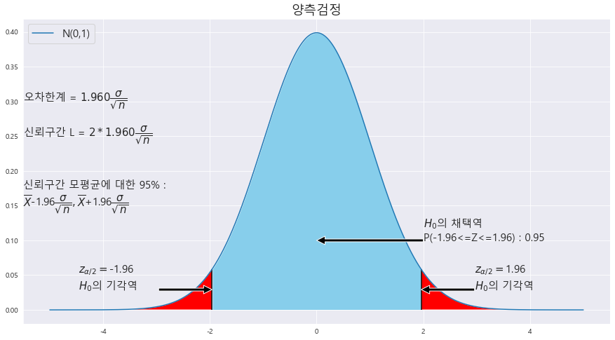
3. 상단측검정(one sided upper hypothesis)
==> 귀무가설 H_0 : Θ <= Θ_0에 대하여 대립가설 H_1 : Θ > Θ_0으로 구성되는 가설 검정이다.
x = np.arange(-5,5 , .001)

fig = plt.figure(figsize=(15,8))
ax = sns.lineplot(x , stats.norm.pdf(x, loc=0 , scale =1)) #정의역 범위 , 평균 = 0 , 표준편차 =1 인 정규분포 플롯

trust = 95 #신뢰도
ax.set_title('상단측검정' ,fontsize = 18)
# z_1 = round((0.05) / math.sqrt( 0.0018532 ) ,2)
# # z_2 = round((34.5 - 35) / math.sqrt(5.5**2 / 25) , 2)
z_1 = round(scipy.stats.norm.ppf(1 - (1-(trust/100))/2) ,3 )

ax.fill_between(x, stats.norm.pdf(x, loc=0 , scale =1) , 0 , where =  (x<=z_1) , facecolor = 'skyblue') # x값 , y값 , 0 , x<=0 인곳 , 색깔

ax.fill_between(x, stats.norm.pdf(x, loc=0 , scale =1) , 0 , where =  (x>=z_1) , facecolor = 'red') # x값 , y값 , 0 , x<=0 인곳 , 색깔


area = scipy.stats.norm.cdf(z_1)
plt.annotate('' , xy=(0, .2), xytext=(2 , .2)  , arrowprops = dict(facecolor = 'black'))

ax.vlines(x= z_1, ymin= 0 , ymax= stats.norm.pdf(z_1, loc=0 , scale =1) , color = 'black' , linestyle ='solid' , label ='{}'.format(2))
# ax.vlines(x= -z_1, ymin= 0 , ymax= stats.norm.pdf(-z_1, loc=0 , scale =1) , color = 'black' , linestyle ='solid' , label ='{}'.format(2))

annotate_len = stats.norm.pdf(z_1, loc=0 , scale =1) /2
plt.annotate('' , xy=(z_1, annotate_len), xytext=(z_1+ 1 , annotate_len)  , arrowprops = dict(facecolor = 'black'))
# plt.annotate('' , xy=(-z_1, annotate_len), xytext=(-1-z_1 , annotate_len)  , arrowprops = dict(facecolor = 'black'))
# ax.text(1 + z_1 , annotate_len , r'$z_{\alpha/2} = $' + f'{round(scipy.stats.norm.ppf(trust/100),3)}\n' + r'$H_{0}$의 기각역',fontsize=15)
ax.text(1 + z_1 , annotate_len+0.02 , r'$z_{\alpha} = $' + f'{z_1}\n' + r'$H_{0}$의 기각역' + f'\nP(Z>={z_1}) = {round(1-area ,3)}',fontsize=15)


ax.text(2 , .2, r'$H_{0}$의 채택역' +f'\nP(Z<={z_1}) : {round(area,4)}',fontsize=15)


MEANS = 60.8
STDS = round(math.sqrt(10.5**2),3) #모표준편차
n = 2490


# ax.text(-5.5 , .35,  r'$\overline{X} = $'+f'{MEANS}\n' + r'$\sigma = $' + f'{STDS}\n' + r'$\sqrt{n} = $' + f'{round(math.sqrt(n),3)}',fontsize=15)

b= 'N(0,1)'

plt.legend([b] , fontsize = 15 , loc='upper left')

# ax.text(-5.5 , .15, f'신뢰구간 모평균에 대한 {trust}% : \n' + r'$\overline{X}$' +f'-{z_1}' + r'$\dfrac{\sigma}{\sqrt{n}},\overline{X}$' + f'+{z_1}' + r'$\dfrac{\sigma}{\sqrt{n}}$ = ' + f'({round(MEANS - z_1*STDS/math.sqrt(n),2)} , {round(MEANS + z_1*STDS/math.sqrt(n),2)})',fontsize=15)
# ax.text(-5.5 , .25,  r'신뢰구간 L = $2*{%.3f}\dfrac{\sigma}{\sqrt{n}} = $' % z_1 + f'{round(2* z_1 * STDS / math.sqrt(n),3)}',fontsize=15)
#
# ax.text(-5.5 , .3,  r'오차한계 = ${%.3f}\dfrac{\sigma}{\sqrt{n}} = $' % z_1 + f'{round(z_1 * STDS / math.sqrt(n),3)}',fontsize=15)

ax.text(-5.5 , .15, f'신뢰구간 모평균에 대한 {trust}% : \n' + r'$\overline{X}$' +f'-{z_1}' + r'$\dfrac{\sigma}{\sqrt{n}},\overline{X}$' + f'+{z_1}' + r'$\dfrac{\sigma}{\sqrt{n}}$ ' ,fontsize=15)
ax.text(-5.5 , .25,  r'신뢰구간 L = $2*{%.3f}\dfrac{\sigma}{\sqrt{n}} $' % z_1 ,fontsize=15)

ax.text(-5.5 , .3,  r'오차한계 = ${%.3f}\dfrac{\sigma}{\sqrt{n}} $' % z_1,fontsize=15)
4. 하단측검정(one sided lower hypothesis)
==> 귀무가설 H_0 : Θ >= Θ_0에 대하여 대립가설 H_1 : Θ < Θ_0으로 구성되는 가설 검정이다.
x = np.arange(-5,5 , .001)

fig = plt.figure(figsize=(15,8))
ax = sns.lineplot(x , stats.norm.pdf(x, loc=0 , scale =1)) #정의역 범위 , 평균 = 0 , 표준편차 =1 인 정규분포 플롯

trust = 95 #신뢰도
ax.set_title('하단측 검정' ,fontsize = 18)
# z_1 = round((0.05) / math.sqrt( 0.0018532 ) ,2)
# # z_2 = round((34.5 - 35) / math.sqrt(5.5**2 / 25) , 2)
z_1 = round(scipy.stats.norm.ppf(1 - (1-(trust/100))/2) ,3 )

ax.fill_between(x, stats.norm.pdf(x, loc=0 , scale =1) , 0 , where =  (x>=-z_1) , facecolor = 'skyblue') # x값 , y값 , 0 , x<=0 인곳 , 색깔

ax.fill_between(x, stats.norm.pdf(x, loc=0 , scale =1) , 0 , where =  (x<=-z_1) , facecolor = 'red') # x값 , y값 , 0 , x<=0 인곳 , 색깔


area = 1- scipy.stats.norm.cdf(-z_1)
plt.annotate('' , xy=(0, .1), xytext=(2 , .1)  , arrowprops = dict(facecolor = 'black'))

# ax.vlines(x= z_1, ymin= 0 , ymax= stats.norm.pdf(z_1, loc=0 , scale =1) , color = 'black' , linestyle ='solid' , label ='{}'.format(2))
ax.vlines(x= -z_1, ymin= 0 , ymax= stats.norm.pdf(-z_1, loc=0 , scale =1) , color = 'black' , linestyle ='solid' , label ='{}'.format(2))

annotate_len = stats.norm.pdf(z_1, loc=0 , scale =1) /2
# plt.annotate('' , xy=(z_1, annotate_len), xytext=(z_1+ 1 , annotate_len)  , arrowprops = dict(facecolor = 'black'))
plt.annotate('' , xy=(-z_1, annotate_len), xytext=(-1-z_1 , annotate_len)  , arrowprops = dict(facecolor = 'black'))
# ax.text(1 + z_1 , annotate_len , r'$z_{\alpha/2} = $' + f'{round(scipy.stats.norm.ppf(trust/100),3)}\n' + r'$H_{0}$의 기각역',fontsize=15)
ax.text(-2.5 - z_1 , annotate_len+0.02 , r'$z_{\alpha} = $' + f'{-z_1}\n' + r'$H_{0}$의 기각역' + f'\nP(Z<={-z_1}) = {round(1-area ,3)}',fontsize=15)


ax.text(2 , .1, r'$H_{0}$의 채택역' +f'\nP({-z_1}<=Z) : {round(area,4)}',fontsize=15)


MEANS = 60.8
STDS = round(math.sqrt(10.5**2),3) #모표준편차
n = 2490


# ax.text(-5.5 , .35,  r'$\overline{X} = $'+f'{MEANS}\n' + r'$\sigma = $' + f'{STDS}\n' + r'$\sqrt{n} = $' + f'{round(math.sqrt(n),3)}',fontsize=15)

b= 'N(0,1)'

plt.legend([b] , fontsize = 15 , loc='upper left')

# ax.text(-5.5 , .15, f'신뢰구간 모평균에 대한 {trust}% : \n' + r'$\overline{X}$' +f'-{z_1}' + r'$\dfrac{\sigma}{\sqrt{n}},\overline{X}$' + f'+{z_1}' + r'$\dfrac{\sigma}{\sqrt{n}}$ = ' + f'({round(MEANS - z_1*STDS/math.sqrt(n),2)} , {round(MEANS + z_1*STDS/math.sqrt(n),2)})',fontsize=15)
# ax.text(-5.5 , .25,  r'신뢰구간 L = $2*{%.3f}\dfrac{\sigma}{\sqrt{n}} = $' % z_1 + f'{round(2* z_1 * STDS / math.sqrt(n),3)}',fontsize=15)
#
# ax.text(-5.5 , .3,  r'오차한계 = ${%.3f}\dfrac{\sigma}{\sqrt{n}} = $' % z_1 + f'{round(z_1 * STDS / math.sqrt(n),3)}',fontsize=15)

ax.text(-5.5 , .15, f'신뢰구간 모평균에 대한 {trust}% : \n' + r'$\overline{X}$' +f'-{z_1}' + r'$\dfrac{\sigma}{\sqrt{n}},\overline{X}$' + f'+{z_1}' + r'$\dfrac{\sigma}{\sqrt{n}}$ ' ,fontsize=15)
ax.text(-5.5 , .25,  r'신뢰구간 L = $2*{%.3f}\dfrac{\sigma}{\sqrt{n}} $' % z_1 ,fontsize=15)

ax.text(-5.5 , .3,  r'오차한계 = ${%.3f}\dfrac{\sigma}{\sqrt{n}} $' % z_1,fontsize=15)
==> 관찰값 z_0이 기각역 안에 놓이면 귀무가설 H_0을 기각시킴
==> 관찰값 z_0이 채택역 안에 놓이면 귀무가설 H_0을 기각시키지 못한다.
'기초통계 > 대표본 가설검정' 카테고리의 다른 글
| ★p-value값★검정통계량의 관찰값★모평균 차의 검정★기초통계학-[통계적 가설검정 -06] (0) | 2023.01.15 |
|---|---|
| ★p-value값★검정통계량의 관찰값★모평균에 대한 상단측 검정★기초통계학-[통계적 가설검정 -05] (0) | 2023.01.13 |
| ★p-value값★검정통계량의 관찰값★모평균에 대한 하단측 검정★기초통계학-[통계적 가설검정 -04] (0) | 2023.01.13 |
| ★양측검정에 따른 p-value 값 산정★표본평균의 정규분포★p-값(p-value)★기초통계학-[통계적 가설검정 -03] (0) | 2023.01.13 |
| ★채택,기각역★제1,2종오류★유의수준★대립가설★귀무가설★가설검정★기초통계학-[통계적 가설검정 -01] (0) | 2023.01.13 |