전체 글
-
★표본비율의 정규분포화★모비율의 가설 검정★기초통계학-[연습문제 03 -11]2023.01.16
★t-분포의 합동표본분산 구하는거 기억하기★모평균 차에 대한 소표본 추정★기초통계학-[소표본 추론-03]
1. 두 모평균 차에 대한 소표본 추정
==> 두 모분산이 알려지지 않았으나 동일하다는 사실을 알고 있는 서로 독립인 두 정규모집단의 모평균의 차에 대한 통계적 추론
EX-01) 배기량이 2000cc인 차량과 3000cc인 차량의 rpm을 조사한 결과 다음 표와 같았다. 2000cc 차량과 3000cc 차량의 평균 rpm의 차에 대한 95% 신뢰구간을 구하라.
A = pd.DataFrame( {'2000cc 차량' : [2360, 2230 , 2350 , 2430 , 2380 , 2360]  , '3000cc 차량' :  [2250 , 2230 , 2300 , 2240 , 2260 , 2340] }).T

A
https://knowallworld.tistory.com/308
★두 표본평균의 차에 대한 표본분포(모분산 모를때)★중심극한정리 활용★이표본의 표본분포
1. 두 표본평균의 차에 대한 표본분포(두 모분산을 모르는 경우) https://knowallworld.tistory.com/302 ★모분산을 모를땐 t-분포!★stats.norm.cdf()★모분산을 알때/모를때 표본평균의 표본분포★일표본 1. 표
knowallworld.tistory.com

X = np.arange(-5,5 , .01)

fig = plt.figure(figsize=(15,15))


#
# A = "1073 1067 1103 1122 1057 1096 1057 1053 1089 1102 1100 1091 1053 1138 1063 1120 1077 1091"
# A = list(map(int, A.split(' ')))


A = [2360, 2330 , 2350 , 2430 , 2380 , 2360]
B = [2250 , 2230 , 2300 , 2240 , 2260 , 2340]


MEANS_A = np.mean(A)
# print(MEANS_A)
STDS_A = np.std(A , ddof=1)
# print(STDS_A**2)
MEANS_B =  np.mean(B)
# print(MEANS_B)
STDS_B = np.std(B , ddof=1)
# print(STDS_B**2)
n_A = len(A) #표본개수
n_B = len(B)
dof = n_A+n_B-2
dof_2 = [dof] #자유도c

MEANS = round(MEANS_A - MEANS_B,4)
STDS = round(math.sqrt(( (n_A-1) * (STDS_A**2) + (n_B-1) * (STDS_B**2))/(dof)),4) # 합동표본표준편차

ax = sns.lineplot(x = X , y=scipy.stats.t(dof_2).pdf(X) )
trust = 95 #신뢰도
trust = round( (1- trust/100)/2 , 4)
t_r =  scipy.stats.t(dof_2).ppf(1- trust)
print(t_r)
t_l = scipy.stats.t(dof_2).ppf(trust)
print(t_l)

E = round(float(t_r * STDS * math.sqrt((1/n_A + 1/n_B))),4)


ax.set_title('두 모평균 차에 대한 소표본 추정' , fontsize = 15)
# =========================================================

ax.fill_between(X, scipy.stats.t(dof_2).pdf(X) , 0 , where = (X<t_r) & (X>t_l) , facecolor = 'orange') # x값 , y값 , 0 , X조건 인곳 , 색깔
ax.fill_between(X, scipy.stats.t(dof_2).pdf(X) , 0 , where = (X>=t_r) | (X<=t_l) , facecolor = 'skyblue') # x값 , y값 , 0 , X조건 인곳 , 색깔
area = round(float(scipy.stats.t(dof_2).cdf(t_r) - scipy.stats.t(dof_2).cdf(t_l)),4)


plt.annotate('' , xy=(0, .2), xytext=(-2.5 , .25)  , arrowprops = dict(facecolor = 'black'))
ax.text(-4.6 , .28, f'평균(MEANS_A - MEANS_B) = {MEANS}\n'  +f' n = {n_A} , m = {n_B}  \n 합동표본분산' +r'$(s^{2})$ = ' + '\n' + r'$S _{p}^{2}=\dfrac{1}{n+m-2}\left[ \left( n-1\right) S _{1}^{2}+\left( m-1\right) S_{2}^{2}\right]$' + f'\n = {STDS}\n' +r'오차한계 $e_{%d} = t_{\dfrac{\alpha}{2}}*{s}*\sqrt{\dfrac{1}{n} + \dfrac{1}{m}}$' % ((1-  trust*2)*100 ) +f'= {E} \n\n' + r'T = $\dfrac{\overline{X} - \overline{Y} - ({\mu}_{1} - {\mu}_{2})}{s_{p} * \sqrt{\dfrac{1}{n} + \dfrac{1}{m}}}$ ~ t(n+m-2)'  ,fontsize=15)

plt.annotate('' , xy=(0, .25), xytext=(1.5 , .25)  , arrowprops = dict(facecolor = 'black'))
ax.text(1.6 , .25, r'$P(t_{%.3f}<T<t_{%.3f})$' % (trust , 1-trust) + f'= {area}\n' + r'신뢰구간 = (MEANS -$e_{\alpha}$ , MEANS + $e_{\alpha}$)' +f'\n' + r' = $({%.4f} - {%.4f} , {%.4f} + {%.4f})$' % (MEANS, E , MEANS , E)  +f'\n' +r'$ = ({%.4f} , {%.4f})$' % (MEANS-E , MEANS+E)  ,fontsize=15)

ax.vlines(x = t_r ,ymin=0 , ymax= scipy.stats.t(dof_2).pdf(t_r) , colors = 'black')
ax.vlines(x = t_l ,ymin=0 , ymax= scipy.stats.t(dof_2).pdf(t_l) , colors = 'black')


plt.annotate('' , xy=(t_r, .007), xytext=(2.5 , .1)  , arrowprops = dict(facecolor = 'black'))
plt.annotate('' , xy=(t_l, .007), xytext=(-3.5 , .1)  , arrowprops = dict(facecolor = 'black'))
ax.text(1.71 , .13, r'$t_{\dfrac{\alpha}{2}} = {%.4f}$' % t_r + '\n' +r'$\dfrac{\alpha}{2}$ =' + f'{round(float(1- scipy.stats.t(dof_2).cdf(t_r)),3)}',fontsize=15)
ax.text(-3.71 , .13, r'$t_{\dfrac{\alpha}{2}} = {%.4f}$' % t_l + '\n' +r'$\dfrac{\alpha}{2}$ =' +f'{round(float(scipy.stats.t(dof_2).cdf(t_l)),3)}',fontsize=15)

ax.text(t_r - 1 , 0.02 , r'$t_r$' + f'= {t_r}'  , fontsize = 13)
ax.text(t_l + .2 , 0.02 , r'$t_l$' + f'= {t_l}'  , fontsize = 13)


#==================================== 가설 검정 ==========================================


# t_1 = round((MEANS - MO_MEAN)/ (STDS / math.sqrt(n)),4)
#
# print(t_1)
# t_1 = abs(t_1)
# area = round(float(scipy.stats.t(dof_2).cdf(-t_1) + 1 - (scipy.stats.t(dof_2).cdf(t_1))),4)
# ax.fill_between(X, scipy.stats.t(dof_2).pdf(X) , 0 , where = (X>=t_1) | (X<=-t_1) , facecolor = 'skyblue') # x값 , y값 , 0 , X조건 인곳 , 색깔
# ax.fill_between(X, scipy.stats.t(dof_2).pdf(X) , 0 , where = (X>=t_r) | (X<=-t_r) , facecolor = 'red') # x값 , y값 , 0 , X조건 인곳 , 색깔
#
# ax.vlines(x= t_1, ymin= 0 , ymax= stats.t(dof_2).pdf(t_1) , color = 'green' , linestyle ='solid' , label ='{}'.format(2))
# ax.vlines(x= -t_1, ymin= 0 , ymax= stats.t(dof_2).pdf(-t_1) , color = 'green' , linestyle ='solid' , label ='{}'.format(2))
#
# annotate_len = stats.t(dof_2).pdf(t_1) /2
# plt.annotate('' , xy=(t_1, annotate_len), xytext=(-t_1/2 , annotate_len)  , arrowprops = dict(facecolor = 'black'))
# plt.annotate('' , xy=(-t_1, annotate_len), xytext=(t_1/2 , annotate_len)  , arrowprops = dict(facecolor = 'black'))
# ax.text(-1.5 , annotate_len+0.03 , f'P-value : \nP(T<={-t_1}) + P(T>={t_1}) \n = {area}',fontsize=15)
#
# mo = '모평균'
#
# ax.text(-4.6 , .22, r'T = $\dfrac{\overline{X} - {\mu}}{\dfrac{s}{\sqrt{n}}}$' + f'= { round((MEANS - MO_MEAN)/(STDS / math.sqrt(n)),4) }' ,fontsize=15)


b = ['t-(n={})'.format(i) for i in dof_2]
plt.legend(b , fontsize = 15)
신뢰구간 = (49.0394 , 147.6272)
EX-02) 시중에서 판매되고 있는 두 회사의 커피에 포함된 카페인의 양을 조사한 결과, 다음 표와 같았다. 두 회사에서 판매하는 커피에 함유된 평균 카페인의 차에 대한 90% 신뢰구간을 구하라.
A = (n = 8 , |X = 109 , s_1 = 루트(4.25) )
B = (m = 6 , |Y = 107 , s_2 = 루트(4.36) )
X = np.arange(-5,5 , .01)

fig = plt.figure(figsize=(15,15))


#
# A = "1073 1067 1103 1122 1057 1096 1057 1053 1089 1102 1100 1091 1053 1138 1063 1120 1077 1091"
# A = list(map(int, A.split(' ')))


# A = [2360, 2330 , 2350 , 2430 , 2380 , 2360]
# B = [2250 , 2230 , 2300 , 2240 , 2260 , 2340]


MEANS_A = 109
# print(MEANS_A)
STDS_A = math.sqrt(4.25)
# print(STDS_A**2)
MEANS_B =  107
# print(MEANS_B)
STDS_B = math.sqrt(4.36)
# print(STDS_B**2)
n_A = 8 #표본개수
n_B = 6
dof = n_A+n_B-2
dof_2 = [dof] #자유도c

MEANS = round(MEANS_A - MEANS_B,4)
STDS = round(math.sqrt(( (n_A-1) * (STDS_A**2) + (n_B-1) * (STDS_B**2))/(dof)),4) # 합동표본표준편차

ax = sns.lineplot(x = X , y=scipy.stats.t(dof_2).pdf(X) )
trust = 90 #신뢰도
trust = round( (1- trust/100)/2 , 4)
t_r =  scipy.stats.t(dof_2).ppf(1- trust)
print(t_r)
t_l = scipy.stats.t(dof_2).ppf(trust)
print(t_l)

E = round(float(t_r * STDS * math.sqrt((1/n_A + 1/n_B))),4)


ax.set_title('두 모평균 차에 대한 소표본 추정' , fontsize = 15)
# =========================================================

ax.fill_between(X, scipy.stats.t(dof_2).pdf(X) , 0 , where = (X<t_r) & (X>t_l) , facecolor = 'orange') # x값 , y값 , 0 , X조건 인곳 , 색깔
ax.fill_between(X, scipy.stats.t(dof_2).pdf(X) , 0 , where = (X>=t_r) | (X<=t_l) , facecolor = 'skyblue') # x값 , y값 , 0 , X조건 인곳 , 색깔
area = round(float(scipy.stats.t(dof_2).cdf(t_r) - scipy.stats.t(dof_2).cdf(t_l)),4)


plt.annotate('' , xy=(0, .2), xytext=(-2.5 , .25)  , arrowprops = dict(facecolor = 'black'))
ax.text(-4.6 , .28, f'평균(MEANS_A - MEANS_B) = {MEANS}\n'  +f' n = {n_A} , m = {n_B}  \n 합동표본분산' +r'$(s^{2})$ = ' + '\n' + r'$S _{p}^{2}=\dfrac{1}{n+m-2}\left[ \left( n-1\right) S _{1}^{2}+\left( m-1\right) S_{2}^{2}\right]$' + f'\n = {STDS}\n' +r'오차한계 $e_{%d} = t_{\dfrac{\alpha}{2}}*{s}*\sqrt{\dfrac{1}{n} + \dfrac{1}{m}}$' % ((1-  trust*2)*100 ) +f'= {E} \n\n' + r'T = $\dfrac{\overline{X} - \overline{Y} - ({\mu}_{1} - {\mu}_{2})}{s_{p} * \sqrt{\dfrac{1}{n} + \dfrac{1}{m}}}$ ~ t(n+m-2)'  ,fontsize=15)

plt.annotate('' , xy=(0, .25), xytext=(1.5 , .25)  , arrowprops = dict(facecolor = 'black'))
ax.text(1.6 , .25, r'$P(t_{%.3f}<T<t_{%.3f})$' % (trust , 1-trust) + f'= {area}\n' + r'신뢰구간 = (MEANS -$e_{\alpha}$ , MEANS + $e_{\alpha}$)' +f'\n' + r' = $({%.4f} - {%.4f} , {%.4f} + {%.4f})$' % (MEANS, E , MEANS , E)  +f'\n' +r'$ = ({%.4f} , {%.4f})$' % (MEANS-E , MEANS+E)  ,fontsize=15)

ax.vlines(x = t_r ,ymin=0 , ymax= scipy.stats.t(dof_2).pdf(t_r) , colors = 'black')
ax.vlines(x = t_l ,ymin=0 , ymax= scipy.stats.t(dof_2).pdf(t_l) , colors = 'black')


plt.annotate('' , xy=(t_r, .007), xytext=(2.5 , .1)  , arrowprops = dict(facecolor = 'black'))
plt.annotate('' , xy=(t_l, .007), xytext=(-3.5 , .1)  , arrowprops = dict(facecolor = 'black'))
ax.text(1.71 , .13, r'$t_{\dfrac{\alpha}{2}} = {%.4f}$' % t_r + '\n' +r'$\dfrac{\alpha}{2}$ =' + f'{round(float(1- scipy.stats.t(dof_2).cdf(t_r)),3)}',fontsize=15)
ax.text(-3.71 , .13, r'$t_{\dfrac{\alpha}{2}} = {%.4f}$' % t_l + '\n' +r'$\dfrac{\alpha}{2}$ =' +f'{round(float(scipy.stats.t(dof_2).cdf(t_l)),3)}',fontsize=15)

ax.text(t_r - 1 , 0.02 , r'$t_r$' + f'= {t_r}'  , fontsize = 13)
ax.text(t_l + .2 , 0.02 , r'$t_l$' + f'= {t_l}'  , fontsize = 13)


#==================================== 가설 검정 ==========================================


# t_1 = round((MEANS - MO_MEAN)/ (STDS / math.sqrt(n)),4)
#
# print(t_1)
# t_1 = abs(t_1)
# area = round(float(scipy.stats.t(dof_2).cdf(-t_1) + 1 - (scipy.stats.t(dof_2).cdf(t_1))),4)
# ax.fill_between(X, scipy.stats.t(dof_2).pdf(X) , 0 , where = (X>=t_1) | (X<=-t_1) , facecolor = 'skyblue') # x값 , y값 , 0 , X조건 인곳 , 색깔
# ax.fill_between(X, scipy.stats.t(dof_2).pdf(X) , 0 , where = (X>=t_r) | (X<=-t_r) , facecolor = 'red') # x값 , y값 , 0 , X조건 인곳 , 색깔
#
# ax.vlines(x= t_1, ymin= 0 , ymax= stats.t(dof_2).pdf(t_1) , color = 'green' , linestyle ='solid' , label ='{}'.format(2))
# ax.vlines(x= -t_1, ymin= 0 , ymax= stats.t(dof_2).pdf(-t_1) , color = 'green' , linestyle ='solid' , label ='{}'.format(2))
#
# annotate_len = stats.t(dof_2).pdf(t_1) /2
# plt.annotate('' , xy=(t_1, annotate_len), xytext=(-t_1/2 , annotate_len)  , arrowprops = dict(facecolor = 'black'))
# plt.annotate('' , xy=(-t_1, annotate_len), xytext=(t_1/2 , annotate_len)  , arrowprops = dict(facecolor = 'black'))
# ax.text(-1.5 , annotate_len+0.03 , f'P-value : \nP(T<={-t_1}) + P(T>={t_1}) \n = {area}',fontsize=15)
#
# mo = '모평균'
#
# ax.text(-4.6 , .22, r'T = $\dfrac{\overline{X} - {\mu}}{\dfrac{s}{\sqrt{n}}}$' + f'= { round((MEANS - MO_MEAN)/(STDS / math.sqrt(n)),4) }' ,fontsize=15)


b = ['t-(n={})'.format(i) for i in dof_2]
plt.legend(b , fontsize = 15)
신뢰구간 = (0.005 , 3.995)
'기초통계 > 소표본 추론' 카테고리의 다른 글
| ★카이제곱분포★모분산에 대한 소표본 추론★기초통계학-[소표본 추론-06] (0) | 2023.01.18 |
|---|---|
| ★쌍체 t-검정★기초통계학-[소표본 추론-05] (0) | 2023.01.17 |
| ★모평균의 차에 대한 소표본 가설검정★기초통계학-[소표본 추론-04] (0) | 2023.01.17 |
| t-분포는 모분산 모를때★t-분포의 모평균에 대한 검정통계량★T-분포에 대한 양측검정★상단측검정★하단측검정★기초통계학-[소표본 추론-02] (0) | 2023.01.17 |
| ★모평균에 대한 소표본 추론★t-분포의 신뢰구간 구하기★기초통계학-[소표본 추론-01] (0) | 2023.01.17 |
https://knowallworld.tistory.com/302
★모분산을 모를땐 t-분포!★stats.norm.cdf()★모분산을 알때/모를때 표본평균의 표본분포★일표본
1. 표본평균의 표본분포(모분산을 아는 경우) ==> 표본평균에 대한 표본분포는 정규분포를 따른다. EX-01) 모평균 100 , 모분산 9인 정규모집단으로부터 크기 25인 표본을 임의로 추출 1> 표본평균 |X
knowallworld.tistory.com

1. t-분포에 대한 양측검정
==> 양측검정의 귀무가설은 '='
EX-01) 리필용 플라스틱 샴푸 용기를 만드는 한 제조 회사가 국내 최대 용량인 1100ml 의 용기를 생산했다고 광고한다. 이를 확인하기 위해서 18개의 용기를 임의로 수거하여 샴푸의 용량을 조사한 결과 다음과 같았다. 이 자료를 이용하여 샴푸 용기 제조 회사의 주장에 대해 유의수준 5%에서 조사하라.
A = "1073 1067 1103 1122 1057 1096 1057 1053 1089 1102 1100 1091 1053 1138 1063 1120 1077 1091"
A = list(map(int, A.split(' ')))
X = np.arange(-5,5 , .01)
fig = plt.figure(figsize=(15,8))
A = "1073 1067 1103 1122 1057 1096 1057 1053 1089 1102 1100 1091 1053 1138 1063 1120 1077 1091"
A = list(map(int, A.split(' ')))
MEANS = round(np.mean(A),4)
STDS = round(np.std(A , ddof =1 ) , 4)
MO_MEAN = 1100
n = len(A) #표본개수
dof_2 = [n-1] #자유도c
ax = sns.lineplot(x = X , y=scipy.stats.t(dof_2).pdf(X) )
trust = 95 #신뢰도
trust = round( (1- trust/100)/2 , 4)
t_r = scipy.stats.t(dof_2).ppf(1- trust)
print(t_r)
t_l = scipy.stats.t(dof_2).ppf(trust)
print(t_l)
E = round(float(t_r * STDS / math.sqrt(n)),4)
# =========================================================
ax.fill_between(X, scipy.stats.t(dof_2).pdf(X) , 0 , where = (X<t_r) & (X>t_l) , facecolor = 'orange') # x값 , y값 , 0 , X조건 인곳 , 색깔
area = round(float(scipy.stats.t(dof_2).cdf(t_r) - scipy.stats.t(dof_2).cdf(t_l)),4)
plt.annotate('' , xy=(0, .2), xytext=(-2.5 , .25) , arrowprops = dict(facecolor = 'black'))
ax.text(-4.6 , .32, f'평균(MEANS) = {MEANS}\n' +f' n = {n} \n 표준편차(s) = {STDS}\n' +r'오차한계 $e_{95\% } = t_{\dfrac{\alpha}{2}}*\dfrac{s}{\sqrt{n}}$'+f'= {E}',fontsize=15)
plt.annotate('' , xy=(0, .25), xytext=(1.5 , .25) , arrowprops = dict(facecolor = 'black'))
ax.text(1.6 , .25, r'$P(t_{%.3f}<T<t_{%.3f})$' % (trust , 1-trust) + f'= {area}\n' + r'신뢰구간 = (MEANS -$e_{\alpha}$ , MEANS + $e_{\alpha}$)' +f'\n' + r' = $({%.4f} - {%.4f} , {%.4f} + {%.4f})$' % (MEANS, E , MEANS , E) +f'\n' +r'$ = ({%.4f} , {%.4f})$' % (MEANS-E , MEANS+E) ,fontsize=15)
ax.vlines(x = t_r ,ymin=0 , ymax= scipy.stats.t(dof_2).pdf(t_r) , colors = 'black')
ax.vlines(x = t_l ,ymin=0 , ymax= scipy.stats.t(dof_2).pdf(t_l) , colors = 'black')
plt.annotate('' , xy=(t_r, .007), xytext=(2.5 , .1) , arrowprops = dict(facecolor = 'black'))
plt.annotate('' , xy=(t_l, .007), xytext=(-3.5 , .1) , arrowprops = dict(facecolor = 'black'))
ax.text(1.71 , .13, r'$t_{\dfrac{\alpha}{2}} = {%.4f}$' % t_r + '\n' +r'$\dfrac{\alpha}{2}$ =' + f'{round(float(1- scipy.stats.t(dof_2).cdf(t_r)),3)}',fontsize=15)
ax.text(-3.71 , .13, r'$t_{\dfrac{\alpha}{2}} = {%.4f}$' % t_l + '\n' +r'$\dfrac{\alpha}{2}$ =' +f'{round(float(scipy.stats.t(dof_2).cdf(t_l)),3)}',fontsize=15)
ax.text(t_r - 1 , 0.02 , r'$t_r$' + f'= {t_r}' , fontsize = 13)
ax.text(t_l + .2 , 0.02 , r'$t_l$' + f'= {t_l}' , fontsize = 13)
#==================================== 가설 검정 ==========================================
t_1 = round((MEANS - MO_MEAN)/ (STDS / math.sqrt(n)),4)
print(t_1)
t_1 = abs(t_1)
area = round(float(scipy.stats.t(dof_2).cdf(-t_1) + 1 - (scipy.stats.t(dof_2).cdf(t_1))),4)
ax.fill_between(X, scipy.stats.t(dof_2).pdf(X) , 0 , where = (X>=t_1) | (X<=-t_1) , facecolor = 'skyblue') # x값 , y값 , 0 , X조건 인곳 , 색깔
ax.fill_between(X, scipy.stats.t(dof_2).pdf(X) , 0 , where = (X>=t_r) | (X<=-t_r) , facecolor = 'red') # x값 , y값 , 0 , X조건 인곳 , 색깔
ax.vlines(x= t_1, ymin= 0 , ymax= stats.t(dof_2).pdf(t_1) , color = 'green' , linestyle ='solid' , label ='{}'.format(2))
ax.vlines(x= -t_1, ymin= 0 , ymax= stats.t(dof_2).pdf(-t_1) , color = 'green' , linestyle ='solid' , label ='{}'.format(2))
annotate_len = stats.t(dof_2).pdf(t_1) /2
plt.annotate('' , xy=(t_1, annotate_len), xytext=(-t_1/2 , annotate_len) , arrowprops = dict(facecolor = 'black'))
plt.annotate('' , xy=(-t_1, annotate_len), xytext=(t_1/2 , annotate_len) , arrowprops = dict(facecolor = 'black'))
ax.text(-1.5 , annotate_len+0.03 , f'P-value : \nP(T<={-t_1}) + P(T>={t_1}) \n = {area}',fontsize=15)
mo = '모평균'
ax.text(-4.6 , .22, r'T = $\dfrac{\overline{X} - {\mu}}{\dfrac{s}{\sqrt{n}}}$' + f'= { round((MEANS - MO_MEAN)/(STDS / math.sqrt(n)),4) }' ,fontsize=15)
b = ['t-(n={})'.format(i) for i in dof_2]
plt.legend(b , fontsize = 15)
p-value : 0.0349
alpha : 0.05
p-value < alpha ==> 0.0349 > 0.05 ==> 귀무가설 H_0 : m = 1100 는 기각한다. 즉 , 유의수준 5%에서 삼퓨 용기 제조회사의 주장은 설득력이 없다.
EX-02) 어느 음료수 제조 회사에서 시판 중인 음료수의 용량이 360mL 라고 한다. 이 음료수 6개를 수거하여 용량을 측정한 결과, 평균 360.6mL, 표준편차 0.74mL 였다. 이 결과를 이용하여 유의수준 10%에서 음료수의 용량을 조사하라.
H_0 : m = 360
X = np.arange(-5,5 , .01)

fig = plt.figure(figsize=(15,8))


#
# A = "1073 1067 1103 1122 1057 1096 1057 1053 1089 1102 1100 1091 1053 1138 1063 1120 1077 1091"
# A = list(map(int, A.split(' ')))


MEANS = 360.6
STDS = 0.74
MO_MEAN = 360


n = 6 #표본개수
dof_2 = [n-1] #자유도c

ax = sns.lineplot(x = X , y=scipy.stats.t(dof_2).pdf(X) )
trust = 90 #신뢰도
trust = round( (1- trust/100)/2 , 4)
t_r =  scipy.stats.t(dof_2).ppf(1- trust)
print(t_r)
t_l = scipy.stats.t(dof_2).ppf(trust)
print(t_l)

E = round(float(t_r * STDS / math.sqrt(n)),4)


# =========================================================

ax.fill_between(X, scipy.stats.t(dof_2).pdf(X) , 0 , where = (X<t_r) & (X>t_l) , facecolor = 'orange') # x값 , y값 , 0 , X조건 인곳 , 색깔
area = round(float(scipy.stats.t(dof_2).cdf(t_r) - scipy.stats.t(dof_2).cdf(t_l)),4)


plt.annotate('' , xy=(0, .2), xytext=(-2.5 , .25)  , arrowprops = dict(facecolor = 'black'))
ax.text(-4.6 , .32, f'평균(MEANS) = {MEANS}\n'  +f' n = {n} \n 표준편차(s) = {STDS}\n' +r'오차한계 $e_{%d} = t_{\dfrac{\alpha}{2}}*\dfrac{s}{\sqrt{n}}$' % ((1-  trust*2)*100 ) +f'= {E}' ,fontsize=15)

plt.annotate('' , xy=(0, .25), xytext=(1.5 , .25)  , arrowprops = dict(facecolor = 'black'))
ax.text(1.6 , .25, r'$P(t_{%.3f}<T<t_{%.3f})$' % (trust , 1-trust) + f'= {area}\n' + r'신뢰구간 = (MEANS -$e_{\alpha}$ , MEANS + $e_{\alpha}$)' +f'\n' + r' = $({%.4f} - {%.4f} , {%.4f} + {%.4f})$' % (MEANS, E , MEANS , E)  +f'\n' +r'$ = ({%.4f} , {%.4f})$' % (MEANS-E , MEANS+E)  ,fontsize=15)

ax.vlines(x = t_r ,ymin=0 , ymax= scipy.stats.t(dof_2).pdf(t_r) , colors = 'black')
ax.vlines(x = t_l ,ymin=0 , ymax= scipy.stats.t(dof_2).pdf(t_l) , colors = 'black')


plt.annotate('' , xy=(t_r, .007), xytext=(2.5 , .1)  , arrowprops = dict(facecolor = 'black'))
plt.annotate('' , xy=(t_l, .007), xytext=(-3.5 , .1)  , arrowprops = dict(facecolor = 'black'))
ax.text(1.71 , .13, r'$t_{\dfrac{\alpha}{2}} = {%.4f}$' % t_r + '\n' +r'$\dfrac{\alpha}{2}$ =' + f'{round(float(1- scipy.stats.t(dof_2).cdf(t_r)),3)}',fontsize=15)
ax.text(-3.71 , .13, r'$t_{\dfrac{\alpha}{2}} = {%.4f}$' % t_l + '\n' +r'$\dfrac{\alpha}{2}$ =' +f'{round(float(scipy.stats.t(dof_2).cdf(t_l)),3)}',fontsize=15)

ax.text(t_r - 1 , 0.02 , r'$t_r$' + f'= {t_r}'  , fontsize = 13)
ax.text(t_l + .2 , 0.02 , r'$t_l$' + f'= {t_l}'  , fontsize = 13)


#==================================== 가설 검정 ==========================================


t_1 = round((MEANS - MO_MEAN)/ (STDS / math.sqrt(n)),4)

print(t_1)
t_1 = abs(t_1)
area = round(float(scipy.stats.t(dof_2).cdf(-t_1) + 1 - (scipy.stats.t(dof_2).cdf(t_1))),4)
ax.fill_between(X, scipy.stats.t(dof_2).pdf(X) , 0 , where = (X>=t_1) | (X<=-t_1) , facecolor = 'skyblue') # x값 , y값 , 0 , X조건 인곳 , 색깔
ax.fill_between(X, scipy.stats.t(dof_2).pdf(X) , 0 , where = (X>=t_r) | (X<=-t_r) , facecolor = 'red') # x값 , y값 , 0 , X조건 인곳 , 색깔

ax.vlines(x= t_1, ymin= 0 , ymax= stats.t(dof_2).pdf(t_1) , color = 'green' , linestyle ='solid' , label ='{}'.format(2))
ax.vlines(x= -t_1, ymin= 0 , ymax= stats.t(dof_2).pdf(-t_1) , color = 'green' , linestyle ='solid' , label ='{}'.format(2))

annotate_len = stats.t(dof_2).pdf(t_1) /2
plt.annotate('' , xy=(t_1, annotate_len), xytext=(-t_1/2 , annotate_len)  , arrowprops = dict(facecolor = 'black'))
plt.annotate('' , xy=(-t_1, annotate_len), xytext=(t_1/2 , annotate_len)  , arrowprops = dict(facecolor = 'black'))
ax.text(-1.5 , annotate_len+0.03 , f'P-value : \nP(T<={-t_1}) + P(T>={t_1}) \n = {area}',fontsize=15)

mo = '모평균'

ax.text(-4.6 , .22, r'T = $\dfrac{\overline{X} - {\mu}}{\dfrac{s}{\sqrt{n}}}$' + f'= { round((MEANS - MO_MEAN)/(STDS / math.sqrt(n)),4) }' ,fontsize=15)


b = ['t-(n={})'.format(i) for i in dof_2]
plt.legend(b , fontsize = 15)
p-value : 0.1038
alpha : 0.1
p-value > alpha ==> 0.1038 > 0.1 ==> 귀무가설 H_0 : m = 360 는 채택한다. 즉 , 유의수준 10%에서 음료수의 용량이 360mL라는 주장은 설득력이 있다.
2. t-분포에 대한 하단측검정
EX-03) 어느 타이어 제조 회사에서 생산된 타이어의 평균 수명이 10이상인지 알아보기 위하여 이 회사의 타이어 10개를 조사한 결과, 평균 9.6 , 표준편차 0.504였다. 이 자료를 이용하여 타이어의 평균 수명이 10 이상인지 유의수준 2.5%에서 조사하라.
H_0 : 평균수명 >= 10
|X = 9.6
s = 0.504
n = 10
X = np.arange(-5,5 , .01)

fig = plt.figure(figsize=(15,8))


#
# A = "1073 1067 1103 1122 1057 1096 1057 1053 1089 1102 1100 1091 1053 1138 1063 1120 1077 1091"
# A = list(map(int, A.split(' ')))


MEANS = 9.6
STDS = 0.504
MO_MEAN = 10


n = 10 #표본개수
dof_2 = [n-1] #자유도c

ax = sns.lineplot(x = X , y=scipy.stats.t(dof_2).pdf(X) )
trust = 97.5 #신뢰도
trust = round( (1- trust/100) , 4)
t_r =  scipy.stats.t(dof_2).ppf(1- trust)
print(t_r)
t_l = scipy.stats.t(dof_2).ppf(trust)
print(t_l)

E = round(float(t_r * STDS / math.sqrt(n)),4) #오차한계


ax.set_title('하단측검정' , fontsize = 15)
# =========================================================

ax.fill_between(X, scipy.stats.t(dof_2).pdf(X) , 0 , where = (X>=-t_r)  , facecolor = 'orange') # x값 , y값 , 0 , X조건 인곳 , 색깔
area = round(float(1- scipy.stats.t(dof_2).cdf(t_l)),4)


plt.annotate('' , xy=(0, .2), xytext=(-2.5 , .25)  , arrowprops = dict(facecolor = 'black'))
ax.text(-4.6 , .32, f'평균(MEANS) = {MEANS}\n'  +f' n = {n} \n 표준편차(s) = {STDS}\n' +r'오차한계 $e_{%d} = t_{{\alpha}}*\dfrac{s}{\sqrt{n}}$' % ((1-  trust)*100 ) +f'= {E}' ,fontsize=15)

plt.annotate('' , xy=(0, .25), xytext=(1.5 , .25)  , arrowprops = dict(facecolor = 'black'))
ax.text(1.6 , .25, r'$P(t_{%.3f}<T)$' % (trust) + f'= {area}\n' + r'신뢰구간 = (MEANS -$e_{\alpha}$ , MEANS + $e_{\alpha}$)' +f'\n' + r' = $({%.4f} - {%.4f} , {%.4f} + {%.4f})$' % (MEANS, E , MEANS , E)  +f'\n' +r'$ = ({%.4f} , {%.4f})$' % (MEANS-E , MEANS+E)  ,fontsize=15)

# ax.vlines(x = t_r ,ymin=0 , ymax= scipy.stats.t(dof_2).pdf(t_r) , colors = 'black')
ax.vlines(x = t_l ,ymin=0 , ymax= scipy.stats.t(dof_2).pdf(t_l) , colors = 'black')


# plt.annotate('' , xy=(t_r, .007), xytext=(2.5 , .1)  , arrowprops = dict(facecolor = 'black'))
plt.annotate('' , xy=(t_l, .007), xytext=(-3.5 , .1)  , arrowprops = dict(facecolor = 'black'))
# ax.text(1.71 , .13, r'$t_{\dfrac{\alpha}{2}} = {%.4f}$' % t_r + '\n' +r'$\dfrac{\alpha}{2}$ =' + f'{round(float(1- scipy.stats.t(dof_2).cdf(t_r)),3)}',fontsize=15)
ax.text(-3.71 , .13, r'$t_{{\alpha}} = {%.4f}$' % t_l + '\n' +r'${\alpha}$ =' +f'{round(float(scipy.stats.t(dof_2).cdf(t_l)),3)}',fontsize=15)

# ax.text(t_r - 1 , 0.02 , r'$t_r$' + f'= {t_r}'  , fontsize = 13)
ax.text(t_l + .2 , 0.02 , r'$t_l$' + f'= {t_l}'  , fontsize = 13)


#==================================== 가설 검정 ==========================================


t_1 = round((MEANS - MO_MEAN)/ (STDS / math.sqrt(n)),4)

print(t_1)
t_1 = abs(t_1)
area = round(float(scipy.stats.t(dof_2).cdf(-t_1) ),4)
ax.fill_between(X, scipy.stats.t(dof_2).pdf(X) , 0 , where =  (X<=-t_1) , facecolor = 'skyblue') # x값 , y값 , 0 , X조건 인곳 , 색깔
ax.fill_between(X, scipy.stats.t(dof_2).pdf(X) , 0 , where = (X<=t_l) , facecolor = 'red') # x값 , y값 , 0 , X조건 인곳 , 색깔

# ax.vlines(x= t_1, ymin= 0 , ymax= stats.t(dof_2).pdf(t_1) , color = 'green' , linestyle ='solid' , label ='{}'.format(2))
ax.vlines(x= -t_1, ymin= 0 , ymax= stats.t(dof_2).pdf(-t_1) , color = 'green' , linestyle ='solid' , label ='{}'.format(2))

annotate_len = stats.t(dof_2).pdf(t_1) /2
# plt.annotate('' , xy=(t_1, annotate_len), xytext=(-t_1/2 , annotate_len)  , arrowprops = dict(facecolor = 'black'))
plt.annotate('' , xy=(-t_1, annotate_len), xytext=(t_1/2 , annotate_len)  , arrowprops = dict(facecolor = 'black'))
ax.text(0.7, annotate_len+0.03 , f'P-value : \nP(T<={-t_1}) \n = {area}',fontsize=15)

mo = '모평균'

ax.text(-4.6 , .22, r'T = $\dfrac{\overline{X} - {\mu}}{\dfrac{s}{\sqrt{n}}}$' + f'= { round((MEANS - MO_MEAN)/(STDS / math.sqrt(n)),4) }' ,fontsize=15)


b = ['t-(n={})'.format(i) for i in dof_2]
plt.legend(b , fontsize = 15)
p-value : 0.0167
alpha : 0.025
p-value < alpha ==> 0.0167 > 0.025 ==> 귀무가설 H_0 : m >= 10(하단측 검정) 은 기각한다. 즉 , 유의수준 2.5%에서 타이어의 평균 수명은 10 이상의 증거가 불충분하다.
EX-04) 뼈와 치아에 가장 중요한 요소 중 하나인 칼슘의 하루 섭취량은 800 mg 이다. 차상위 계층 이하인 사람들의 하루 섭취량이 이 기준에 미치지 못하는지 알아보기 위하여 6명의 차상위 계층 이하인 사람을 임의로 선정하여 조사한 결과, 평균 774 mg , 표준편차 31.4mg 이었다. 이 자료를 이용하여 차상위 계층 이하인 사람들의 하루 칼슘 섭취량의 미달 여부를 유의수준 5%에서 조사하라.
|X = 774
s = 31.4
n = 6
H_0 : M >= 800
X = np.arange(-5,5 , .01)

fig = plt.figure(figsize=(15,8))


#
# A = "1073 1067 1103 1122 1057 1096 1057 1053 1089 1102 1100 1091 1053 1138 1063 1120 1077 1091"
# A = list(map(int, A.split(' ')))


MEANS = 774
STDS = 31.4
MO_MEAN = 800


n = 6 #표본개수
dof_2 = [n-1] #자유도c

ax = sns.lineplot(x = X , y=scipy.stats.t(dof_2).pdf(X) )
trust = 95 #신뢰도
trust = round( (1- trust/100) , 4)
t_r =  scipy.stats.t(dof_2).ppf(1- trust)
print(t_r)
t_l = scipy.stats.t(dof_2).ppf(trust)
print(t_l)

E = round(float(t_r * STDS / math.sqrt(n)),4) #오차한계


ax.set_title('하단측검정' , fontsize = 15)
# =========================================================

ax.fill_between(X, scipy.stats.t(dof_2).pdf(X) , 0 , where = (X>=-t_r)  , facecolor = 'orange') # x값 , y값 , 0 , X조건 인곳 , 색깔
area = round(float(1- scipy.stats.t(dof_2).cdf(t_l)),4)


plt.annotate('' , xy=(0, .2), xytext=(-2.5 , .25)  , arrowprops = dict(facecolor = 'black'))
ax.text(-4.6 , .32, f'평균(MEANS) = {MEANS}\n'  +f' n = {n} \n 표준편차(s) = {STDS}\n' +r'오차한계 $e_{%d} = t_{{\alpha}}*\dfrac{s}{\sqrt{n}}$' % ((1-  trust)*100 ) +f'= {E}' ,fontsize=15)

plt.annotate('' , xy=(0, .25), xytext=(1.5 , .25)  , arrowprops = dict(facecolor = 'black'))
ax.text(1.6 , .25, r'$P(t_{%.3f}<T)$' % (trust) + f'= {area}\n' + r'신뢰구간 = (MEANS -$e_{\alpha}$ , MEANS + $e_{\alpha}$)' +f'\n' + r' = $({%.4f} - {%.4f} , {%.4f} + {%.4f})$' % (MEANS, E , MEANS , E)  +f'\n' +r'$ = ({%.4f} , {%.4f})$' % (MEANS-E , MEANS+E)  ,fontsize=15)

# ax.vlines(x = t_r ,ymin=0 , ymax= scipy.stats.t(dof_2).pdf(t_r) , colors = 'black')
ax.vlines(x = t_l ,ymin=0 , ymax= scipy.stats.t(dof_2).pdf(t_l) , colors = 'black')


# plt.annotate('' , xy=(t_r, .007), xytext=(2.5 , .1)  , arrowprops = dict(facecolor = 'black'))
plt.annotate('' , xy=(t_l, .007), xytext=(-3.5 , .1)  , arrowprops = dict(facecolor = 'black'))
# ax.text(1.71 , .13, r'$t_{\dfrac{\alpha}{2}} = {%.4f}$' % t_r + '\n' +r'$\dfrac{\alpha}{2}$ =' + f'{round(float(1- scipy.stats.t(dof_2).cdf(t_r)),3)}',fontsize=15)
ax.text(-3.71 , .13, r'$t_{{\alpha}} = {%.4f}$' % t_l + '\n' +r'${\alpha}$ =' +f'{round(float(scipy.stats.t(dof_2).cdf(t_l)),3)}',fontsize=15)

# ax.text(t_r - 1 , 0.02 , r'$t_r$' + f'= {t_r}'  , fontsize = 13)
ax.text(t_l + .2 , 0.02 , r'$t_l$' + f'= {t_l}'  , fontsize = 13)


#==================================== 가설 검정 ==========================================


t_1 = round((MEANS - MO_MEAN)/ (STDS / math.sqrt(n)),4)

print(t_1)
t_1 = abs(t_1)
area = round(float(scipy.stats.t(dof_2).cdf(-t_1) ),4)
ax.fill_between(X, scipy.stats.t(dof_2).pdf(X) , 0 , where =  (X<=-t_1) , facecolor = 'skyblue') # x값 , y값 , 0 , X조건 인곳 , 색깔
ax.fill_between(X, scipy.stats.t(dof_2).pdf(X) , 0 , where = (X<=t_l) , facecolor = 'red') # x값 , y값 , 0 , X조건 인곳 , 색깔

# ax.vlines(x= t_1, ymin= 0 , ymax= stats.t(dof_2).pdf(t_1) , color = 'green' , linestyle ='solid' , label ='{}'.format(2))
ax.vlines(x= -t_1, ymin= 0 , ymax= stats.t(dof_2).pdf(-t_1) , color = 'green' , linestyle ='solid' , label ='{}'.format(2))

annotate_len = stats.t(dof_2).pdf(t_1) /2
# plt.annotate('' , xy=(t_1, annotate_len), xytext=(-t_1/2 , annotate_len)  , arrowprops = dict(facecolor = 'black'))
plt.annotate('' , xy=(-t_1, annotate_len), xytext=(t_1/2 , annotate_len)  , arrowprops = dict(facecolor = 'black'))
ax.text(0.7, annotate_len+0.03 , f'P-value : \nP(T<={-t_1}) \n = {area}',fontsize=15)

mo = '모평균'

ax.text(-4.6 , .22, r'T = $\dfrac{\overline{X} - {\mu}}{\dfrac{s}{\sqrt{n}}}$' + f'= { round((MEANS - MO_MEAN)/(STDS / math.sqrt(n)),4) }' ,fontsize=15)


b = ['t-(n={})'.format(i) for i in dof_2]
plt.legend(b , fontsize = 15)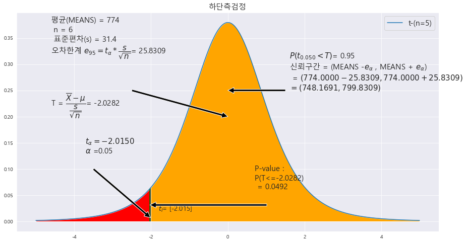
p-value : 0.0492
alpha : 0.05
p-value < alpha ==> 0.0492 < 0.05 ==> 귀무가설 H_0 : M >= 800(하단측 검정) 은 기각한다. 즉 , 유의수준 5%에서 칼슘의 섭취량이 800mg 에 부족하다.
3. t-분포에 대한 상단측검정
EX-05) 어느 대형 마트를 이용하는 고객의 지출이 1인당 평균 9만원을 초과하는지 알아보기 위하여 임의로 고객 6명을 선정하여 조사한 결과 다음과 같았다. 이마트에서 1인당 지출이 9만 원을 초과하는지 유의수준 5%에서 조사하라.
[14.8, 9.5, 11.2, 9.8, 10.2, 9.4]
H_0 : m <= 9(상단측 검정)
MEANS = 10.8167
n = 6
s = 2.0576
X = np.arange(-5,5 , .01)

fig = plt.figure(figsize=(15,8))


#
A = "14.8 9.5 11.2 9.8 10.2 9.4"
A = list(map(float, A.split(' ')))
print(A)

MEANS = round(np.mean(A) , 4)
STDS = round(np.std(A , ddof =1 ) ,4)
MO_MEAN = 9


n = len(A) #표본개수
dof_2 = [n-1] #자유도c

ax = sns.lineplot(x = X , y=scipy.stats.t(dof_2).pdf(X) )
trust = 95 #신뢰도
trust = round( (1- trust/100) , 4)
t_r =  scipy.stats.t(dof_2).ppf(1- trust)
print(t_r)
t_l = scipy.stats.t(dof_2).ppf(trust)
print(t_l)

E = round(float(t_r * STDS / math.sqrt(n)),4) #오차한계


ax.set_title('상단측검정' , fontsize = 15)
# =========================================================

ax.fill_between(X, scipy.stats.t(dof_2).pdf(X) , 0 , where = (X<=t_r)  , facecolor = 'orange') # x값 , y값 , 0 , X조건 인곳 , 색깔
area = round(float(scipy.stats.t(dof_2).cdf(t_r)),4)


plt.annotate('' , xy=(0, .2), xytext=(-2.5 , .25)  , arrowprops = dict(facecolor = 'black'))
ax.text(-4.6 , .32, f'평균(MEANS) = {MEANS}\n'  +f' n = {n} \n 표준편차(s) = {STDS}\n' +r'오차한계 $e_{%d} = t_{{\alpha}}*\dfrac{s}{\sqrt{n}}$' % ((1-  trust)*100 ) +f'= {E}' ,fontsize=15)

plt.annotate('' , xy=(0, .25), xytext=(1.5 , .25)  , arrowprops = dict(facecolor = 'black'))
ax.text(1.6 , .25, r'$P(t_{%.3f}>T)$' % (trust) + f'= {area}\n' + r'신뢰구간 = (MEANS -$e_{\alpha}$ , MEANS + $e_{\alpha}$)' +f'\n' + r' = $({%.4f} - {%.4f} , {%.4f} + {%.4f})$' % (MEANS, E , MEANS , E)  +f'\n' +r'$ = ({%.4f} , {%.4f})$' % (MEANS-E , MEANS+E)  ,fontsize=15)

# ax.vlines(x = t_r ,ymin=0 , ymax= scipy.stats.t(dof_2).pdf(t_r) , colors = 'black')
ax.vlines(x = t_r ,ymin=0 , ymax= scipy.stats.t(dof_2).pdf(t_r) , colors = 'black')


# plt.annotate('' , xy=(t_r, .007), xytext=(2.5 , .1)  , arrowprops = dict(facecolor = 'black'))
plt.annotate('' , xy=(t_r, .007), xytext=(2.5 , .1)  , arrowprops = dict(facecolor = 'black'))
# ax.text(1.71 , .13, r'$t_{\dfrac{\alpha}{2}} = {%.4f}$' % t_r + '\n' +r'$\dfrac{\alpha}{2}$ =' + f'{round(float(1- scipy.stats.t(dof_2).cdf(t_r)),3)}',fontsize=15)
ax.text(2.71 , .13, r'$t_{{\alpha}} = {%.4f}$' % t_r + '\n' +r'${\alpha}$ =' +f'{round(float(1- scipy.stats.t(dof_2).cdf(t_r)),3)}',fontsize=15)

ax.text(t_r - 1 , 0.02 , r'$t_r$' + f'= {t_r}'  , fontsize = 13)
# ax.text(t_l + .2 , 0.02 , r'$t_l$' + f'= {t_l}'  , fontsize = 13)


#==================================== 가설 검정 ==========================================


t_1 = round((MEANS - MO_MEAN)/ (STDS / math.sqrt(n)),4)

print(t_1)
t_1 = abs(t_1)
area = round(1- float(scipy.stats.t(dof_2).cdf(t_1) ),4)
ax.fill_between(X, scipy.stats.t(dof_2).pdf(X) , 0 , where =  (X>=t_1) , facecolor = 'skyblue') # x값 , y값 , 0 , X조건 인곳 , 색깔
ax.fill_between(X, scipy.stats.t(dof_2).pdf(X) , 0 , where = (X>=t_r) , facecolor = 'red') # x값 , y값 , 0 , X조건 인곳 , 색깔

ax.vlines(x= t_1, ymin= 0 , ymax= stats.t(dof_2).pdf(t_1) , color = 'green' , linestyle ='solid' , label ='{}'.format(2))
# ax.vlines(x= -t_1, ymin= 0 , ymax= stats.t(dof_2).pdf(-t_1) , color = 'green' , linestyle ='solid' , label ='{}'.format(2))

annotate_len = stats.t(dof_2).pdf(t_1) /2
plt.annotate('' , xy=(t_1, annotate_len), xytext=(-t_1/2 , annotate_len)  , arrowprops = dict(facecolor = 'black'))
# plt.annotate('' , xy=(-t_1, annotate_len), xytext=(t_1/2 , annotate_len)  , arrowprops = dict(facecolor = 'black'))
ax.text(-1.5, annotate_len+0.03 , f'P-value : \nP(T>={t_1}) \n = {area}',fontsize=15)

mo = '모평균'

ax.text(-4.6 , .22, r'T = $\dfrac{\overline{X} - {\mu}}{\dfrac{s}{\sqrt{n}}}$' + f'= { round((MEANS - MO_MEAN)/(STDS / math.sqrt(n)),4) }' ,fontsize=15)


b = ['t-(n={})'.format(i) for i in dof_2]
plt.legend(b , fontsize = 15)
p-value : 0.0415
alpha : 0.05
p-value < alpha ==> 0.0415 < 0.05 ==> 귀무가설 H_0 : m<= 9(상단측 검정) 은 기각한다. 즉 , 유의수준 5%에서 고객의 1인당 지출액이 9만원을 초과한다.
EX-06) 스마트폰에 사용되는 베터리의 수명이 하루를 초과하는지 알아보기 위하여 10개를 임의로 선정하여 조사한 결과, 평균 1.2일 , 표준편차 0.35일 이었다. 배터리의 수명이 하루를 초과하는지 유의수준 5%에서 조사하라.
H_0 : m<= 1 (상단측검정)
|X = 1.2
s = 0.35
n = 10
X = np.arange(-5,5 , .01)

fig = plt.figure(figsize=(15,8))


#
# A = "14.8 9.5 11.2 9.8 10.2 9.4"
# A = list(map(float, A.split(' ')))
# print(A)

MEANS = 1.2
STDS = 0.35
MO_MEAN = 1


n = 10 #표본개수
dof_2 = [n-1] #자유도c

ax = sns.lineplot(x = X , y=scipy.stats.t(dof_2).pdf(X) )
trust = 95 #신뢰도
trust = round( (1- trust/100) , 4)
t_r =  scipy.stats.t(dof_2).ppf(1- trust)
print(t_r)
t_l = scipy.stats.t(dof_2).ppf(trust)
print(t_l)

E = round(float(t_r * STDS / math.sqrt(n)),4) #오차한계


ax.set_title('상단측검정' , fontsize = 15)
# =========================================================

ax.fill_between(X, scipy.stats.t(dof_2).pdf(X) , 0 , where = (X<=t_r)  , facecolor = 'orange') # x값 , y값 , 0 , X조건 인곳 , 색깔
area = round(float(scipy.stats.t(dof_2).cdf(t_r)),4)


plt.annotate('' , xy=(0, .2), xytext=(-2.5 , .25)  , arrowprops = dict(facecolor = 'black'))
ax.text(-4.6 , .32, f'평균(MEANS) = {MEANS}\n'  +f' n = {n} \n 표준편차(s) = {STDS}\n' +r'오차한계 $e_{%d} = t_{{\alpha}}*\dfrac{s}{\sqrt{n}}$' % ((1-  trust)*100 ) +f'= {E}' ,fontsize=15)

plt.annotate('' , xy=(0, .25), xytext=(1.5 , .25)  , arrowprops = dict(facecolor = 'black'))
ax.text(1.6 , .25, r'$P(t_{%.3f}>T)$' % (trust) + f'= {area}\n' + r'신뢰구간 = (MEANS -$e_{\alpha}$ , MEANS + $e_{\alpha}$)' +f'\n' + r' = $({%.4f} - {%.4f} , {%.4f} + {%.4f})$' % (MEANS, E , MEANS , E)  +f'\n' +r'$ = ({%.4f} , {%.4f})$' % (MEANS-E , MEANS+E)  ,fontsize=15)

# ax.vlines(x = t_r ,ymin=0 , ymax= scipy.stats.t(dof_2).pdf(t_r) , colors = 'black')
ax.vlines(x = t_r ,ymin=0 , ymax= scipy.stats.t(dof_2).pdf(t_r) , colors = 'black')


# plt.annotate('' , xy=(t_r, .007), xytext=(2.5 , .1)  , arrowprops = dict(facecolor = 'black'))
plt.annotate('' , xy=(t_r, .007), xytext=(2.5 , .1)  , arrowprops = dict(facecolor = 'black'))
# ax.text(1.71 , .13, r'$t_{\dfrac{\alpha}{2}} = {%.4f}$' % t_r + '\n' +r'$\dfrac{\alpha}{2}$ =' + f'{round(float(1- scipy.stats.t(dof_2).cdf(t_r)),3)}',fontsize=15)
ax.text(2.71 , .13, r'$t_{{\alpha}} = {%.4f}$' % t_r + '\n' +r'${\alpha}$ =' +f'{round(float(1- scipy.stats.t(dof_2).cdf(t_r)),3)}',fontsize=15)

ax.text(t_r - 1 , 0.02 , r'$t_r$' + f'= {t_r}'  , fontsize = 13)
# ax.text(t_l + .2 , 0.02 , r'$t_l$' + f'= {t_l}'  , fontsize = 13)


#==================================== 가설 검정 ==========================================


t_1 = round((MEANS - MO_MEAN)/ (STDS / math.sqrt(n)),4)

print(t_1)
t_1 = abs(t_1)
area = round(1- float(scipy.stats.t(dof_2).cdf(t_1) ),4)
ax.fill_between(X, scipy.stats.t(dof_2).pdf(X) , 0 , where =  (X>=t_1) , facecolor = 'skyblue') # x값 , y값 , 0 , X조건 인곳 , 색깔
ax.fill_between(X, scipy.stats.t(dof_2).pdf(X) , 0 , where = (X>=t_r) , facecolor = 'red') # x값 , y값 , 0 , X조건 인곳 , 색깔

ax.vlines(x= t_1, ymin= 0 , ymax= stats.t(dof_2).pdf(t_1) , color = 'green' , linestyle ='solid' , label ='{}'.format(2))
# ax.vlines(x= -t_1, ymin= 0 , ymax= stats.t(dof_2).pdf(-t_1) , color = 'green' , linestyle ='solid' , label ='{}'.format(2))

annotate_len = stats.t(dof_2).pdf(t_1) /2
plt.annotate('' , xy=(t_1, annotate_len), xytext=(-t_1/2 , annotate_len)  , arrowprops = dict(facecolor = 'black'))
# plt.annotate('' , xy=(-t_1, annotate_len), xytext=(t_1/2 , annotate_len)  , arrowprops = dict(facecolor = 'black'))
ax.text(-1.5, annotate_len+0.03 , f'P-value : \nP(T>={t_1}) \n = {area}',fontsize=15)

mo = '모평균'

ax.text(-4.6 , .22, r'T = $\dfrac{\overline{X} - {\mu}}{\dfrac{s}{\sqrt{n}}}$' + f'= { round((MEANS - MO_MEAN)/(STDS / math.sqrt(n)),4) }' ,fontsize=15)


b = ['t-(n={})'.format(i) for i in dof_2]
plt.legend(b , fontsize = 15)
p-value : 0.0521
alpha : 0.05
p-value > alpha ==> 0.0521 > 0.05 ==> 귀무가설 H_0 : m<= 1(상단측 검정) 은 채택한다. 즉 , 배터리의 수명이 하루를 초과한다는 증거는 부족하다.
4. p-value 검정
EX-07) 어느 광역시의 보건환경연구원이 해당 광역시 주요 도로의 질소산화물은 위험수준인 0.101ppm보다 작다고 주장하였다. 이를 알아보기 위하여 이 지역의 주요 도로 18곳의 질소산화물 배출을 조사한 결과, 평균 0.098ppm , 표준편차 0.005 ppm이었다. p-value 값을 구하여 보건환경연구원의 주장에 대해 유의수준 1%에서 조사하라.
H_0 : m >= 0.101(하단측 검정)
|X = 0.098
s = 0.005
n = 18
X = np.arange(-5,5 , .01)

fig = plt.figure(figsize=(15,8))


#
# A = "1073 1067 1103 1122 1057 1096 1057 1053 1089 1102 1100 1091 1053 1138 1063 1120 1077 1091"
# A = list(map(int, A.split(' ')))


MEANS = 0.098
STDS = 0.005
MO_MEAN = 0.101


n = 18 #표본개수
dof_2 = [n-1] #자유도c

ax = sns.lineplot(x = X , y=scipy.stats.t(dof_2).pdf(X) )
trust = 99 #신뢰도
trust = round( (1- trust/100) , 4)
t_r =  scipy.stats.t(dof_2).ppf(1- trust)
print(t_r)
t_l = scipy.stats.t(dof_2).ppf(trust)
print(t_l)

E = round(float(t_r * STDS / math.sqrt(n)),4) #오차한계


ax.set_title('하단측검정' , fontsize = 15)
# =========================================================

ax.fill_between(X, scipy.stats.t(dof_2).pdf(X) , 0 , where = (X>=-t_r)  , facecolor = 'orange') # x값 , y값 , 0 , X조건 인곳 , 색깔
area = round(float(1- scipy.stats.t(dof_2).cdf(t_l)),4)


plt.annotate('' , xy=(0, .2), xytext=(-2.5 , .25)  , arrowprops = dict(facecolor = 'black'))
ax.text(-4.6 , .32, f'평균(MEANS) = {MEANS}\n'  +f' n = {n} \n 표준편차(s) = {STDS}\n' +r'오차한계 $e_{%d} = t_{{\alpha}}*\dfrac{s}{\sqrt{n}}$' % ((1-  trust)*100 ) +f'= {E}' ,fontsize=15)

plt.annotate('' , xy=(0, .25), xytext=(1.5 , .25)  , arrowprops = dict(facecolor = 'black'))
ax.text(1.6 , .25, r'$P(t_{%.3f}<T)$' % (trust) + f'= {area}\n' + r'신뢰구간 = (MEANS -$e_{\alpha}$ , MEANS + $e_{\alpha}$)' +f'\n' + r' = $({%.4f} - {%.4f} , {%.4f} + {%.4f})$' % (MEANS, E , MEANS , E)  +f'\n' +r'$ = ({%.4f} , {%.4f})$' % (MEANS-E , MEANS+E)  ,fontsize=15)

# ax.vlines(x = t_r ,ymin=0 , ymax= scipy.stats.t(dof_2).pdf(t_r) , colors = 'black')
ax.vlines(x = t_l ,ymin=0 , ymax= scipy.stats.t(dof_2).pdf(t_l) , colors = 'black')


# plt.annotate('' , xy=(t_r, .007), xytext=(2.5 , .1)  , arrowprops = dict(facecolor = 'black'))
plt.annotate('' , xy=(t_l, .007), xytext=(-3.5 , .1)  , arrowprops = dict(facecolor = 'black'))
# ax.text(1.71 , .13, r'$t_{\dfrac{\alpha}{2}} = {%.4f}$' % t_r + '\n' +r'$\dfrac{\alpha}{2}$ =' + f'{round(float(1- scipy.stats.t(dof_2).cdf(t_r)),3)}',fontsize=15)
ax.text(-3.71 , .13, r'$t_{{\alpha}} = {%.4f}$' % t_l + '\n' +r'${\alpha}$ =' +f'{round(float(scipy.stats.t(dof_2).cdf(t_l)),3)}',fontsize=15)

# ax.text(t_r - 1 , 0.02 , r'$t_r$' + f'= {t_r}'  , fontsize = 13)
ax.text(t_l + .2 , 0.02 , r'$t_l$' + f'= {t_l}'  , fontsize = 13)


#==================================== 가설 검정 ==========================================


t_1 = round((MEANS - MO_MEAN)/ (STDS / math.sqrt(n)),4)

print(t_1)
t_1 = abs(t_1)
area = round(float(scipy.stats.t(dof_2).cdf(-t_1) ),4)
ax.fill_between(X, scipy.stats.t(dof_2).pdf(X) , 0 , where =  (X<=-t_1) , facecolor = 'skyblue') # x값 , y값 , 0 , X조건 인곳 , 색깔
ax.fill_between(X, scipy.stats.t(dof_2).pdf(X) , 0 , where = (X<=t_l) , facecolor = 'red') # x값 , y값 , 0 , X조건 인곳 , 색깔

# ax.vlines(x= t_1, ymin= 0 , ymax= stats.t(dof_2).pdf(t_1) , color = 'green' , linestyle ='solid' , label ='{}'.format(2))
ax.vlines(x= -t_1, ymin= 0 , ymax= stats.t(dof_2).pdf(-t_1) , color = 'green' , linestyle ='solid' , label ='{}'.format(2))

annotate_len = stats.t(dof_2).pdf(t_1) /2
# plt.annotate('' , xy=(t_1, annotate_len), xytext=(-t_1/2 , annotate_len)  , arrowprops = dict(facecolor = 'black'))
plt.annotate('' , xy=(-t_1, annotate_len), xytext=(t_1/2 , annotate_len)  , arrowprops = dict(facecolor = 'black'))
ax.text(0.7, annotate_len+0.03 , f'P-value : \nP(T<={-t_1}) \n = {area}',fontsize=15)

mo = '모평균'

ax.text(-4.6 , .22, r'T = $\dfrac{\overline{X} - {\mu}}{\dfrac{s}{\sqrt{n}}}$' + f'= { round((MEANS - MO_MEAN)/(STDS / math.sqrt(n)),4) }' ,fontsize=15)


b = ['t-(n={})'.format(i) for i in dof_2]
plt.legend(b , fontsize = 15)
p-value : 0.0104
alpha : 0.01
p-value > alpha ==> 0.0104 > 0.01 ==> 귀무가설 H_0 : m>= 0.101(하단측 검정) 은 채택한다. 즉 , 주요도로의 위험수준은 0.101보다 크거나 같다.
EX-08) 모평균이 m<= 10이라는 주장에 대한 타당성을 조사하기 위하여 크기 25인 표본을 조사한 결과, 표본평균 10.3과 표본표준편차 2를 얻었다. p-value 값을 구하고 유의수준 5%에서 검정하라.
H_0 : m<=10 (상단측 검정)
|X = 10.3
s = 2
n = 25
X = np.arange(-5,5 , .01)

fig = plt.figure(figsize=(15,8))


#
# A = "14.8 9.5 11.2 9.8 10.2 9.4"
# A = list(map(float, A.split(' ')))
# print(A)

MEANS = 10.3
STDS = 2
MO_MEAN = 10


n = 25 #표본개수
dof_2 = [n-1] #자유도c

ax = sns.lineplot(x = X , y=scipy.stats.t(dof_2).pdf(X) )
trust = 95 #신뢰도
trust = round( (1- trust/100) , 4)
t_r =  scipy.stats.t(dof_2).ppf(1- trust)
print(t_r)
t_l = scipy.stats.t(dof_2).ppf(trust)
print(t_l)

E = round(float(t_r * STDS / math.sqrt(n)),4) #오차한계


ax.set_title('상단측검정' , fontsize = 15)
# =========================================================

ax.fill_between(X, scipy.stats.t(dof_2).pdf(X) , 0 , where = (X<=t_r)  , facecolor = 'orange') # x값 , y값 , 0 , X조건 인곳 , 색깔
area = round(float(scipy.stats.t(dof_2).cdf(t_r)),4)


plt.annotate('' , xy=(0, .2), xytext=(-2.5 , .25)  , arrowprops = dict(facecolor = 'black'))
ax.text(-4.6 , .32, f'평균(MEANS) = {MEANS}\n'  +f' n = {n} \n 표준편차(s) = {STDS}\n' +r'오차한계 $e_{%d} = t_{{\alpha}}*\dfrac{s}{\sqrt{n}}$' % ((1-  trust)*100 ) +f'= {E}' ,fontsize=15)

plt.annotate('' , xy=(0, .25), xytext=(1.5 , .25)  , arrowprops = dict(facecolor = 'black'))
ax.text(1.6 , .25, r'$P(t_{%.3f}>T)$' % (trust) + f'= {area}\n' + r'신뢰구간 = (MEANS -$e_{\alpha}$ , MEANS + $e_{\alpha}$)' +f'\n' + r' = $({%.4f} - {%.4f} , {%.4f} + {%.4f})$' % (MEANS, E , MEANS , E)  +f'\n' +r'$ = ({%.4f} , {%.4f})$' % (MEANS-E , MEANS+E)  ,fontsize=15)

# ax.vlines(x = t_r ,ymin=0 , ymax= scipy.stats.t(dof_2).pdf(t_r) , colors = 'black')
ax.vlines(x = t_r ,ymin=0 , ymax= scipy.stats.t(dof_2).pdf(t_r) , colors = 'black')


# plt.annotate('' , xy=(t_r, .007), xytext=(2.5 , .1)  , arrowprops = dict(facecolor = 'black'))
plt.annotate('' , xy=(t_r, .007), xytext=(2.5 , .1)  , arrowprops = dict(facecolor = 'black'))
# ax.text(1.71 , .13, r'$t_{\dfrac{\alpha}{2}} = {%.4f}$' % t_r + '\n' +r'$\dfrac{\alpha}{2}$ =' + f'{round(float(1- scipy.stats.t(dof_2).cdf(t_r)),3)}',fontsize=15)
ax.text(2.71 , .13, r'$t_{{\alpha}} = {%.4f}$' % t_r + '\n' +r'${\alpha}$ =' +f'{round(float(1- scipy.stats.t(dof_2).cdf(t_r)),3)}',fontsize=15)

ax.text(t_r - 1 , 0.02 , r'$t_r$' + f'= {t_r}'  , fontsize = 13)
# ax.text(t_l + .2 , 0.02 , r'$t_l$' + f'= {t_l}'  , fontsize = 13)


#==================================== 가설 검정 ==========================================


t_1 = round((MEANS - MO_MEAN)/ (STDS / math.sqrt(n)),4)

print(t_1)
t_1 = abs(t_1)
area = round(1- float(scipy.stats.t(dof_2).cdf(t_1) ),4)
ax.fill_between(X, scipy.stats.t(dof_2).pdf(X) , 0 , where =  (X>=t_1) , facecolor = 'skyblue') # x값 , y값 , 0 , X조건 인곳 , 색깔
ax.fill_between(X, scipy.stats.t(dof_2).pdf(X) , 0 , where = (X>=t_r) , facecolor = 'red') # x값 , y값 , 0 , X조건 인곳 , 색깔

ax.vlines(x= t_1, ymin= 0 , ymax= stats.t(dof_2).pdf(t_1) , color = 'green' , linestyle ='solid' , label ='{}'.format(2))
# ax.vlines(x= -t_1, ymin= 0 , ymax= stats.t(dof_2).pdf(-t_1) , color = 'green' , linestyle ='solid' , label ='{}'.format(2))

annotate_len = stats.t(dof_2).pdf(t_1) /2
plt.annotate('' , xy=(t_1, annotate_len), xytext=(-t_1/2 , annotate_len)  , arrowprops = dict(facecolor = 'black'))
# plt.annotate('' , xy=(-t_1, annotate_len), xytext=(t_1/2 , annotate_len)  , arrowprops = dict(facecolor = 'black'))
ax.text(-1.5, annotate_len+0.03 , f'P-value : \nP(T>={t_1}) \n = {area}',fontsize=15)

mo = '모평균'

ax.text(-4.6 , .22, r'T = $\dfrac{\overline{X} - {\mu}}{\dfrac{s}{\sqrt{n}}}$' + f'= { round((MEANS - MO_MEAN)/(STDS / math.sqrt(n)),4) }' ,fontsize=15)


b = ['t-(n={})'.format(i) for i in dof_2]
plt.legend(b , fontsize = 15)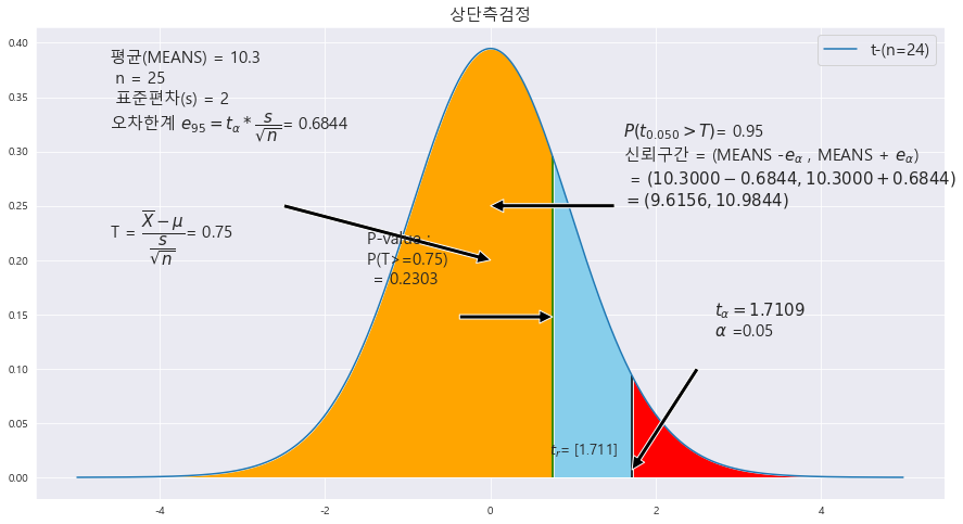
p-value : 0.2303
alpha : 0.05
p-value > alpha ==> 0.2303 > 0.01 ==> 귀무가설 H_0 : m<= 10(상단측 검정) 은 채택한다. 즉 , 모평균은 10보 다 작거나 같다.
'기초통계 > 소표본 추론' 카테고리의 다른 글
| ★카이제곱분포★모분산에 대한 소표본 추론★기초통계학-[소표본 추론-06] (0) | 2023.01.18 |
|---|---|
| ★쌍체 t-검정★기초통계학-[소표본 추론-05] (0) | 2023.01.17 |
| ★모평균의 차에 대한 소표본 가설검정★기초통계학-[소표본 추론-04] (0) | 2023.01.17 |
| ★t-분포의 합동표본분산 구하는거 기억하기★모평균 차에 대한 소표본 추정★기초통계학-[소표본 추론-03] (0) | 2023.01.17 |
| ★모평균에 대한 소표본 추론★t-분포의 신뢰구간 구하기★기초통계학-[소표본 추론-01] (0) | 2023.01.17 |
★모평균에 대한 소표본 추론★t-분포의 신뢰구간 구하기★기초통계학-[소표본 추론-01]
1. 모평균에 대한 소표본 추정
==> 대표본인 경우 , 모분산을 알고 있는 정규모집단 또는 모분산을 모르지만 대표본을 이용한 모집단의 모평균을 추론하는 방법 살펴보았다.
==> 모분산을 알고 있는 정규모집단인 경우에는 표본의 크기에 관계없이 정규분포를 사용하였다.
==> but. 대부분 모집단은 모분산이 알려져 있지 않다.
==> 모분산을 모르고 표본의 크기가 작은 경우에 모평균을 추정하거나 검정하는 통계적 추론을 살펴볼 필요가 있다.
https://knowallworld.tistory.com/302
★모분산을 모를땐 t-분포!★stats.norm.cdf()★모분산을 알때/모를때 표본평균의 표본분포★일표본
1. 표본평균의 표본분포(모분산을 아는 경우) ==> 표본평균에 대한 표본분포는 정규분포를 따른다. EX-01) 모평균 100 , 모분산 9인 정규모집단으로부터 크기 25인 표본을 임의로 추출 1> 표본평균 |X
knowallworld.tistory.com
==> 모표준편차가 알려지지 않은 경우에 표본평균 |X의 표준화에서 모표준편차를 표본표준편차 s로 대치하면, |X의 표준화 확률변수는 자유도가 n-1인 t-분포를 따른다.
EX-01) 정규모집단에서 크기 10인 표본을 추출하여 조사
A = [3.1 , 1.9 , 2.4 , 2.8 , 2.9 , 3.0 , 2.8 , 2.3, 2.2 , 2.6]

print(f'평균 : {np.mean(A)}')

print(f'표본분산 : {np.var(A ,ddof=1)}')


print(f'표본표준편차 : {np.std(A ,ddof=1)}')
평균 : 2.6
표본분산 : 0.1511111111111111
표본표준편차(s) : 0.3887
==> 모분산 모른다 ==> t-분포 활용
X = np.arange(-5,5 , .01)

fig = plt.figure(figsize=(15,8))


A = [3.1 , 1.9 , 2.4 , 2.8 , 2.9 , 3.0 , 2.8 , 2.3, 2.2 , 2.6]

MEANS = round(np.mean(A),4)
STDS = round(np.std(A , ddof=1) ,4)


n = 10 #표본개수
dof_2 = [n-1] #자유도c

ax = sns.lineplot(x = X , y=scipy.stats.t(dof_2).pdf(X) )
trust = 95 #신뢰도
trust = round( (1- trust/100)/2 , 4)
t_r =  scipy.stats.t(dof_2).ppf(1- trust)
print(t_r)
t_l = scipy.stats.t(dof_2).ppf(trust)
print(t_l)

E = round(float(t_r * STDS / math.sqrt(n)),4)


# =========================================================
ax.fill_between(X, scipy.stats.t(dof_2).pdf(X) , 0 , where = (X>=t_r) | (X<=t_l) , facecolor = 'skyblue') # x값 , y값 , 0 , X조건 인곳 , 색깔
ax.fill_between(X, scipy.stats.t(dof_2).pdf(X) , 0 , where = (X<t_r) & (X>t_l) , facecolor = 'orange') # x값 , y값 , 0 , X조건 인곳 , 색깔
area = round(float(scipy.stats.t(dof_2).cdf(t_r) - scipy.stats.t(dof_2).cdf(t_l)),4)


plt.annotate('' , xy=(0, .2), xytext=(-2.5 , .25)  , arrowprops = dict(facecolor = 'black'))
ax.text(-4.6 , .27, f'평균(MEANS) = {MEANS}\n alpha = {round(1-area,4)}\n' + r'$t_{\dfrac{\alpha}{2}} = {%.4f}$' % t_r +f'\n n = {n} \n 표준편차(s) = {STDS}\n' +r'오차한계 $e_{95\% } = t_{\dfrac{\alpha}{2}}*\dfrac{s}{\sqrt{n}}$'+f'= {E}',fontsize=15)

plt.annotate('' , xy=(0, .25), xytext=(1.5 , .25)  , arrowprops = dict(facecolor = 'black'))
ax.text(1.6 , .25, r'$P(t_{%.3f}<T<t_{%.3f})$' % (trust , 1-trust) + f'= {area}\n' + r'신뢰구간 = (MEANS -$e_{\alpha}$ , MEANS + $e_{\alpha}$)' +f'\n' + r' = $({%.4f} - {%.4f} , {%.4f} + {%.4f})$' % (MEANS, E , MEANS , E)  +f'\n' +r'$ = ({%.4f} , {%.4f})$' % (MEANS-E , MEANS+E)  ,fontsize=15)

ax.vlines(x = t_r ,ymin=0 , ymax= scipy.stats.t(dof_2).pdf(t_r) , colors = 'black')
ax.vlines(x = t_l ,ymin=0 , ymax= scipy.stats.t(dof_2).pdf(t_l) , colors = 'black')

plt.annotate('' , xy=(3.0, .007), xytext=(2.5 , .1)  , arrowprops = dict(facecolor = 'black'))
plt.annotate('' , xy=(-3.0, .007), xytext=(-3.5 , .1)  , arrowprops = dict(facecolor = 'black'))

ax.text(1.71 , .13, r'$P(T>t_{%.3f})$' % trust + f'= {round(float(1- scipy.stats.t(dof_2).cdf(t_r)),3)}',fontsize=15)
ax.text(-3.71 , .13, r'$P(T<t_{%.3f})$' % trust + f'= {round(float(scipy.stats.t(dof_2).cdf(t_l)),3)}',fontsize=15)

ax.text(t_r - 1 , 0.02 , r'$t_r$' + f'= {t_r}'  , fontsize = 13)
ax.text(t_l + .2 , 0.02 , r'$t_l$' + f'= {t_l}'  , fontsize = 13)


b = ['t-(n={})'.format(i) for i in dof_2]
plt.legend(b , fontsize = 15)
==> (2.3219 , 2.8781)
EX-02) 정규모집단에서 크기 17인 표본을 추출하여 조사한 결과 , 표본평균 41 , 표본표준편차 3.2였다. 이때 | |X - m | 에 대한 95% 오차한계와 모평균에 대한 95% 신뢰구간을 구하라.
X = np.arange(-5,5 , .01)

fig = plt.figure(figsize=(15,8))


MEANS = 41
STDS = 3.2


n = 17 #표본개수
dof_2 = [n-1] #자유도c

ax = sns.lineplot(x = X , y=scipy.stats.t(dof_2).pdf(X) )
trust = 95 #신뢰도
trust = round( (1- trust/100)/2 , 4)
t_r =  scipy.stats.t(dof_2).ppf(1- trust)
print(t_r)
t_l = scipy.stats.t(dof_2).ppf(trust)
print(t_l)

E = round(float(t_r * STDS / math.sqrt(n)),4)


# =========================================================
ax.fill_between(X, scipy.stats.t(dof_2).pdf(X) , 0 , where = (X>=t_r) | (X<=t_l) , facecolor = 'skyblue') # x값 , y값 , 0 , X조건 인곳 , 색깔
ax.fill_between(X, scipy.stats.t(dof_2).pdf(X) , 0 , where = (X<t_r) & (X>t_l) , facecolor = 'orange') # x값 , y값 , 0 , X조건 인곳 , 색깔
area = round(float(scipy.stats.t(dof_2).cdf(t_r) - scipy.stats.t(dof_2).cdf(t_l)),4)


plt.annotate('' , xy=(0, .2), xytext=(-2.5 , .25)  , arrowprops = dict(facecolor = 'black'))
ax.text(-4.6 , .27, f'평균(MEANS) = {MEANS}\n alpha = {round(1-area,4)}\n' + r'$t_{\dfrac{\alpha}{2}} = {%.4f}$' % t_r +f'\n n = {n} \n 표준편차(s) = {STDS}\n' +r'오차한계 $e_{95\% } = t_{\dfrac{\alpha}{2}}*\dfrac{s}{\sqrt{n}}$'+f'= {E}',fontsize=15)

plt.annotate('' , xy=(0, .25), xytext=(1.5 , .25)  , arrowprops = dict(facecolor = 'black'))
ax.text(1.6 , .25, r'$P(t_{%.3f}<T<t_{%.3f})$' % (trust , 1-trust) + f'= {area}\n' + r'신뢰구간 = (MEANS -$e_{\alpha}$ , MEANS + $e_{\alpha}$)' +f'\n' + r' = $({%.4f} - {%.4f} , {%.4f} + {%.4f})$' % (MEANS, E , MEANS , E)  +f'\n' +r'$ = ({%.4f} , {%.4f})$' % (MEANS-E , MEANS+E)  ,fontsize=15)

ax.vlines(x = t_r ,ymin=0 , ymax= scipy.stats.t(dof_2).pdf(t_r) , colors = 'black')
ax.vlines(x = t_l ,ymin=0 , ymax= scipy.stats.t(dof_2).pdf(t_l) , colors = 'black')

plt.annotate('' , xy=(3.0, .007), xytext=(2.5 , .1)  , arrowprops = dict(facecolor = 'black'))
plt.annotate('' , xy=(-3.0, .007), xytext=(-3.5 , .1)  , arrowprops = dict(facecolor = 'black'))

ax.text(1.71 , .13, r'$P(T>t_{%.3f})$' % trust + f'= {round(float(1- scipy.stats.t(dof_2).cdf(t_r)),3)}',fontsize=15)
ax.text(-3.71 , .13, r'$P(T<t_{%.3f})$' % trust + f'= {round(float(scipy.stats.t(dof_2).cdf(t_l)),3)}',fontsize=15)

ax.text(t_r - 1 , 0.02 , r'$t_r$' + f'= {t_r}'  , fontsize = 13)
ax.text(t_l + .2 , 0.02 , r'$t_l$' + f'= {t_l}'  , fontsize = 13)


b = ['t-(n={})'.format(i) for i in dof_2]
plt.legend(b , fontsize = 15)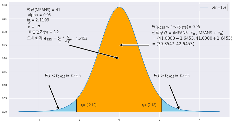
==> (39.3547 , 42.6453)
'기초통계 > 소표본 추론' 카테고리의 다른 글
| ★카이제곱분포★모분산에 대한 소표본 추론★기초통계학-[소표본 추론-06] (0) | 2023.01.18 |
|---|---|
| ★쌍체 t-검정★기초통계학-[소표본 추론-05] (0) | 2023.01.17 |
| ★모평균의 차에 대한 소표본 가설검정★기초통계학-[소표본 추론-04] (0) | 2023.01.17 |
| ★t-분포의 합동표본분산 구하는거 기억하기★모평균 차에 대한 소표본 추정★기초통계학-[소표본 추론-03] (0) | 2023.01.17 |
| t-분포는 모분산 모를때★t-분포의 모평균에 대한 검정통계량★T-분포에 대한 양측검정★상단측검정★하단측검정★기초통계학-[소표본 추론-02] (0) | 2023.01.17 |
★표본비율의 차에 따른 검정★합동표본비율★표본분산 모를때는 표본비율의 차로 검정★기초통계학-[연습문제 06 -14]
23. 남녀 직장인이 받는 스트레스에 대해 조사한 결과가 다음과 같다. 이것을 근거로 남녀 직장인이 받는 스트레스에 차이가 있는지 유의수준 5%에서 조사하라.
https://knowallworld.tistory.com/343
★합동표본비율★양측검정, 상단측검정, 하단측검정 구분하기★모비율 차의 검정★기초통계학-
https://knowallworld.tistory.com/334 ★모평균 , 모비율의 차에 대한 신뢰구간★모비율에 대한 오차한계 및 신뢰구간★기초통계학-[ 16. 2014년에 초,중,고 학생 116000명을 대상으로 우리나라 통일에 대해
knowallworld.tistory.com
A = pd.DataFrame(columns = ['조사인원' , '스트레스를 받은 인원' ] , index = ['남자' , '여자'])
A['조사인원'] = [1650 , 1235 ]
A['스트레스를 받은 인원'] = [1137, 806]
A
H_0 : p_1 = p_2 (양측검정)
x = np.arange(-5,5 , .001)
fig = plt.figure(figsize=(15,8))
ax = sns.lineplot(x , stats.norm.pdf(x, loc=0 , scale =1)) #정의역 범위 , 평균 = 0 , 표준편차 =1 인 정규분포 플롯
# trust = 95 #신뢰도
ax.set_title('양측검정' ,fontsize = 18)
p1 = 1137/1650
p2 = 806/1235
n = 1650
m = 1235
RATIO = round(p1 - p2,4)
print(RATIO)
SAMPLE_PROP = (1137 + 806) / (n+m) #합동표본비율
STDS = math.sqrt( SAMPLE_PROP * (1-SAMPLE_PROP) * (1/n + 1/m))
print(STDS)
#==========================================귀무가설 기각과 채택 ====================================================
trust = 95 #신뢰도_유의수준
t_1 = round(scipy.stats.norm.ppf(1 - (1-(trust/100))) ,3 )
ax.fill_between(x, stats.norm.pdf(x, loc=0 , scale =1) , 0 , where = (x<=t_1) & (x>=-t_1) , facecolor = 'orange') # x값 , y값 , 0 , x<=0 인곳 , 색깔
area = 1- (1- scipy.stats.norm.cdf(t_1))
plt.annotate('' , xy=(0, .2), xytext=(2 , .2) , arrowprops = dict(facecolor = 'black'))
ax.text(2 , .2, r'$H_{0}$의 채택역' +f'\nP({-t_1}<=Z<={t_1}) : {round(area,4)}',fontsize=15)
annotate_len = stats.norm.pdf(t_1, loc=0 , scale =1) /2
ax.vlines(x= t_1, ymin= 0 , ymax= stats.norm.pdf(t_1, loc=0 , scale =1) , color = 'green' , linestyle ='solid' , label ='{}'.format(2))
ax.vlines(x= -t_1, ymin= 0 , ymax= stats.norm.pdf(-t_1, loc=0 , scale =1) , color = 'green' , linestyle ='solid' , label ='{}'.format(2))
area = round((1-area)/2,6)
ax.text(1 + t_1 , annotate_len+0.02 , r'$z_{\alpha/2} = $' + f'{t_1}\n' + r'$H_{0}$의 기각역' + f'\n'+ r'$\alpha/2 = {%.4f}$' % area,fontsize=15)
ax.text(-2.5 -t_1 , annotate_len , r'$z_{\alpha/2} = $' + f'{-t_1}\n' + r'$H_{0}$의 기각역' + f'\n'+ r'$\alpha/2 = {%.3f}$' % area,fontsize=15)
plt.annotate('' , xy=(t_1, annotate_len-0.02), xytext=(t_1+ 1 , annotate_len) , arrowprops = dict(facecolor = 'black'))
plt.annotate('' , xy=(-t_1, annotate_len-0.02), xytext=(-1-t_1 , annotate_len) , arrowprops = dict(facecolor = 'black'))
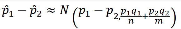
ax.text(-5.5 , .25, f'신뢰구간 모평균에 대한 {trust}% : \n' + r'$\left(\widehat{p}_{1} - \widehat{p}_{2}\right)$' +f'-{t_1}' + r'$\sqrt{\dfrac{\widehat{p}_{1}\widehat{q}_{1}}{n}+\dfrac{\widehat{p}_{2}\widehat{q}_{2}}{m}}$' +' , \n'+ r'$\left(\widehat{p}_{1} - \widehat{p}_{2}\right)$' +f'+ {t_1}' + r'$\sqrt{\dfrac{\widehat{p}_{1}\widehat{q}_{1}}{n}+\dfrac{\widehat{p}_{2}\widehat{q}_{2}}{m}}$',fontsize=15)
ax.text(-5.5 , .15, f'신뢰구간 모비율간 차에 대한 {trust}%의 합동표본비율 : \n' + r'$Z = \dfrac{\widehat{p}_1 - \widehat{p}_2}{ \sqrt{\widehat{p}\widehat{q} * (\dfrac{1}{n} + \dfrac{1}{m}}) }$' + f'= { round((p1 - p2) / math.sqrt(SAMPLE_PROP * (1-SAMPLE_PROP) * ( (1 / n) + (1/m))),4) }',fontsize=15)
ax.text(2 , .35 , r'합동표본비율의 $ \widehat{p} = \dfrac{x + y}{n + m}$' ,fontsize= 15)
# ax.text(-5.5 , .25, f'귀무가설 : 남자(u_1)의 입원일수가 여자(u_2)의 입원일수 보다 작다.\n u_1 < u_2' , fontsize = 15)
# ax.text(1 , .35, f' 신뢰구간 {trust}% 에 대한 오차 한계( ' +r'$e_{%d}) : $ '% trust + f'\n' + r'${%.3f}\sqrt{\dfrac{\widehat{p}_{1}\widehat{q}_{1}}{n}+\dfrac{\widehat{p}_{2}\widehat{q}_{2}}{m}}$ = '% t_1 + f'{round((t_1)*math.sqrt(p1*(1-p1)/n + p2*(1-p2)/m),3)} ' , fontsize= 15)
# ax.text(-5.5 , .25, r'신뢰구간 L = $2*{%.3f}\dfrac{\sigma}{\sqrt{n}} $' % t_1 ,fontsize=15)
#
# ax.text(-5.5 , .3, r'오차한계 = ${%.3f}\dfrac{\sigma}{\sqrt{n}} $' % t_1,fontsize=15)
#============================================표본평균의 정규분포화 =========================================================
z_1 = round(RATIO/STDS , 4)
print(z_1)
# # z_2 = round((34.5 - 35) / math.sqrt(5.5**2 / 25) , 2)
# z_1 = round(scipy.stats.norm.ppf(1 - (1-(trust/100))/2) ,3 )
ax.fill_between(x, stats.norm.pdf(x, loc=0 , scale =1) , 0 , where = (x>=z_1) | (x<=-z_1) , facecolor = 'skyblue') # x값 , y값 , 0 , x<=0 인곳 , 색깔
ax.fill_between(x, stats.norm.pdf(x, loc=0 , scale =1) , 0 , where = (x>=t_1) | (x<=-t_1) , facecolor = 'red') # x값 , y값 , 0 , x<=0 인곳 , 색깔
area = scipy.stats.norm.cdf(-z_1) + 1 - (scipy.stats.norm.cdf(z_1))
ax.vlines(x= z_1, ymin= 0 , ymax= stats.norm.pdf(z_1, loc=0 , scale =1) , color = 'black' , linestyle ='solid' , label ='{}'.format(2))
ax.vlines(x= -z_1, ymin= 0 , ymax= stats.norm.pdf(-z_1, loc=0 , scale =1) , color = 'black' , linestyle ='solid' , label ='{}'.format(2))
annotate_len = stats.norm.pdf(z_1, loc=0 , scale =1) /2
plt.annotate('' , xy=(z_1, annotate_len), xytext=(-z_1/2 , annotate_len) , arrowprops = dict(facecolor = 'black'))
plt.annotate('' , xy=(-z_1, annotate_len), xytext=(z_1/2 , annotate_len) , arrowprops = dict(facecolor = 'black'))
ax.text(-1.5 , annotate_len+0.01 , f'P-value : \nP(Z<={-z_1}) + P(Z>={z_1}) \n = {round(area,4)}',fontsize=15)
# ax.text(0 , annotate_len+0.01 ,f'P(Z>={-z_1})',fontsize=15)
b= 'N(0,1)'
plt.legend([b] , fontsize = 15 , loc='upper left')
P-value = 0.0386
alpha = 0.05
귀무가설 H_0 : 남자의 스트레스 = 여자의 스트레스
p-value < alpha ==> 0.0386 < 0.05 ==> 귀무가설 기각 ==> 남자의 스트레스와 여자의 스트레스는 동일하지 않다.
24. A와 B 두 도시 간, 특정 정당 지지율에 차이가 있는지 알아보기 위하여 두 도시에서 500명씩 임의로 추출하여 지지도를 조사한 결과, A 도시에서 275명, B 도시에서 244명이 지지하는 것으로 조사되었다. 이 자료를 근거로 두 도시 간의 지지도에 차이가 있는지 유의수준 5%에서 조사하라.
^p_A = 275/500
^p_B = 244/500
==> 표준편차 모른다. ==> 표본비율간 차이에 따른 검정 시행
H_0 : p_A = p_B(양측검정)
x = np.arange(-5,5 , .001)

fig = plt.figure(figsize=(15,8))
ax = sns.lineplot(x , stats.norm.pdf(x, loc=0 , scale =1)) #정의역 범위 , 평균 = 0 , 표준편차 =1 인 정규분포 플롯

# trust = 95 #신뢰도

ax.set_title('양측검정' ,fontsize = 18)
p1 = 275/500
p2 = 244/500

n = 500
m = 500

RATIO = round(p1 - p2,4)
print(RATIO)
SAMPLE_PROP = (275 + 244) / (n+m) #합동표본비율

STDS = math.sqrt( SAMPLE_PROP * (1-SAMPLE_PROP) * (1/n + 1/m))
print(STDS)


#==========================================귀무가설 기각과 채택 ====================================================
trust = 95 #신뢰도_유의수준

t_1  = round(scipy.stats.norm.ppf(1 - (1-(trust/100))) ,3 )


ax.fill_between(x, stats.norm.pdf(x, loc=0 , scale =1) , 0 , where = (x<=t_1) & (x>=-t_1) , facecolor = 'orange') # x값 , y값 , 0 , x<=0 인곳 , 색깔
area = 1- (1- scipy.stats.norm.cdf(t_1))

plt.annotate('' , xy=(0, .2), xytext=(2 , .2)  , arrowprops = dict(facecolor = 'black'))
ax.text(2 , .2, r'$H_{0}$의 채택역' +f'\nP({-t_1}<=Z<={t_1}) : {round(area,4)}',fontsize=15)

annotate_len = stats.norm.pdf(t_1, loc=0 , scale =1) /2
ax.vlines(x= t_1, ymin= 0 , ymax= stats.norm.pdf(t_1, loc=0 , scale =1) , color = 'green' , linestyle ='solid' , label ='{}'.format(2))
ax.vlines(x= -t_1, ymin= 0 , ymax= stats.norm.pdf(-t_1, loc=0 , scale =1) , color = 'green' , linestyle ='solid' , label ='{}'.format(2))
area = round((1-area)/2,6)
ax.text(1 + t_1 , annotate_len+0.02 , r'$z_{\alpha/2} = $' + f'{t_1}\n' + r'$H_{0}$의 기각역' + f'\n'+ r'$\alpha/2 = {%.4f}$' % area,fontsize=15)
ax.text(-2.5 -t_1 , annotate_len , r'$z_{\alpha/2} = $' + f'{-t_1}\n' + r'$H_{0}$의 기각역' + f'\n'+ r'$\alpha/2 = {%.3f}$' % area,fontsize=15)


plt.annotate('' , xy=(t_1, annotate_len-0.02), xytext=(t_1+ 1 , annotate_len)  , arrowprops = dict(facecolor = 'black'))
plt.annotate('' , xy=(-t_1, annotate_len-0.02), xytext=(-1-t_1 , annotate_len)  , arrowprops = dict(facecolor = 'black'))


ax.text(-5.5 , .25, f'신뢰구간 모평균에 대한 {trust}% : \n' + r'$\left(\widehat{p}_{1} - \widehat{p}_{2}\right)$' +f'-{t_1}' + r'$\sqrt{\dfrac{\widehat{p}_{1}\widehat{q}_{1}}{n}+\dfrac{\widehat{p}_{2}\widehat{q}_{2}}{m}}$' +' , \n'+ r'$\left(\widehat{p}_{1} - \widehat{p}_{2}\right)$' +f'+ {t_1}' + r'$\sqrt{\dfrac{\widehat{p}_{1}\widehat{q}_{1}}{n}+\dfrac{\widehat{p}_{2}\widehat{q}_{2}}{m}}$',fontsize=15)

ax.text(-5.5 , .15, f'신뢰구간 모비율간 차에 대한 {trust}%의 합동표본비율 : \n' + r'$Z = \dfrac{\widehat{p}_1 - \widehat{p}_2}{ \sqrt{\widehat{p}\widehat{q} * (\dfrac{1}{n} + \dfrac{1}{m}})  }$' + f'=  { round((p1 - p2) / math.sqrt(SAMPLE_PROP * (1-SAMPLE_PROP) * ( (1 / n) + (1/m))),4) }',fontsize=15)

ax.text(2 , .35 , r'합동표본비율의 $ \widehat{p} = \dfrac{x + y}{n + m}$' ,fontsize= 15)

# ax.text(-5.5 , .25, f'귀무가설 : 남자(u_1)의 입원일수가 여자(u_2)의 입원일수 보다 작다.\n u_1 < u_2'  , fontsize = 15)
# ax.text(1 , .35, f' 신뢰구간 {trust}% 에 대한 오차 한계( ' +r'$e_{%d}) : $ '% trust + f'\n' + r'${%.3f}\sqrt{\dfrac{\widehat{p}_{1}\widehat{q}_{1}}{n}+\dfrac{\widehat{p}_{2}\widehat{q}_{2}}{m}}$ = '% t_1 + f'{round((t_1)*math.sqrt(p1*(1-p1)/n + p2*(1-p2)/m),3)} ' , fontsize= 15)


# ax.text(-5.5 , .25,  r'신뢰구간 L = $2*{%.3f}\dfrac{\sigma}{\sqrt{n}} $' % t_1 ,fontsize=15)
#
# ax.text(-5.5 , .3,  r'오차한계 = ${%.3f}\dfrac{\sigma}{\sqrt{n}} $' % t_1,fontsize=15)


#============================================표본평균의 정규분포화 =========================================================

z_1 = round(RATIO/STDS  , 4)
print(z_1)
# # z_2 = round((34.5 - 35) / math.sqrt(5.5**2 / 25) , 2)
# z_1 = round(scipy.stats.norm.ppf(1 - (1-(trust/100))/2) ,3 )

ax.fill_between(x, stats.norm.pdf(x, loc=0 , scale =1) , 0 , where = (x>=z_1) | (x<=-z_1) , facecolor = 'skyblue') # x값 , y값 , 0 , x<=0 인곳 , 색깔
ax.fill_between(x, stats.norm.pdf(x, loc=0 , scale =1) , 0 , where = (x>=t_1) | (x<=-t_1) , facecolor = 'red') # x값 , y값 , 0 , x<=0 인곳 , 색깔
area =  scipy.stats.norm.cdf(-z_1) + 1 - (scipy.stats.norm.cdf(z_1))


ax.vlines(x= z_1, ymin= 0 , ymax= stats.norm.pdf(z_1, loc=0 , scale =1) , color = 'black' , linestyle ='solid' , label ='{}'.format(2))
ax.vlines(x= -z_1, ymin= 0 , ymax= stats.norm.pdf(-z_1, loc=0 , scale =1) , color = 'black' , linestyle ='solid' , label ='{}'.format(2))

annotate_len = stats.norm.pdf(z_1, loc=0 , scale =1) /2
plt.annotate('' , xy=(z_1, annotate_len), xytext=(-z_1/2 , annotate_len)  , arrowprops = dict(facecolor = 'black'))
plt.annotate('' , xy=(-z_1, annotate_len), xytext=(z_1/2 , annotate_len)  , arrowprops = dict(facecolor = 'black'))
ax.text(-1.5 , annotate_len+0.01 , f'P-value : \nP(Z<={-z_1}) + P(Z>={z_1}) \n = {round(area,4)}',fontsize=15)
# ax.text(0 , annotate_len+0.01 ,f'P(Z>={-z_1})',fontsize=15)


b= 'N(0,1)'

plt.legend([b] , fontsize = 15 , loc='upper left')

P-value = 0.0498
alpha = 0.05
귀무가설 H_0 : 두 도시간 지지도에 차이가 없다.
p-value < alpha ==> 0.0498 < 0.05 ==> 귀무가설 기각 ==> 두 도시간 지지도에 차이가 있다.
25. 어떤 단체에서 국영 TV의 광고 방송에 대한 찬반을 묻는 조사를 실시하였다. 대도시에 거주하는 사람들 2055명중 1312명이 찬성하였고, 농어촌에 거주하는 사람 800명 중 486명이 찬성하였다. 도시 사람의 찬성률이 농어촌 사람의 찬성률 보다 큰지 유의수준 5%에서 조사하라.
^p_1 = 1312/2055
^p_2 = 486/800
p1 > p2
==> H_0 : p_1 <= p_2 (상단측 검정)
x = np.arange(-5,5 , .001)

fig = plt.figure(figsize=(15,8))
ax = sns.lineplot(x , stats.norm.pdf(x, loc=0 , scale =1)) #정의역 범위 , 평균 = 0 , 표준편차 =1 인 정규분포 플롯

# trust = 95 #신뢰도
p1 = 1312/2055
p2 = 486/800

n = 2055
m = 800


ax.set_title('상단측검정' ,fontsize = 18)
RATIO = round(p1 - p2,4)
SAMPLE_PROP = (1312 + 486) / (n+m) #합동표본비율

#==========================================귀무가설 기각과 채택 ====================================================
trust = 95 #신뢰도_유의수준

t_1  = round(scipy.stats.norm.ppf(1-(1-(trust/100))) ,3 )


ax.fill_between(x, stats.norm.pdf(x, loc=0 , scale =1) , 0 , where =  (x<=t_1) , facecolor = 'orange') # x값 , y값 , 0 , x<=0 인곳 , 색깔
area = scipy.stats.norm.cdf(t_1)

plt.annotate('' , xy=(0, .2), xytext=(2 , .2)  , arrowprops = dict(facecolor = 'black'))
ax.text(2 , .2, r'$H_{0}$의 채택역' +f'\nP(Z<={t_1}) : {round(area,4)}',fontsize=15)

annotate_len = stats.norm.pdf(t_1, loc=0 , scale =1) /2
ax.vlines(x= t_1, ymin= 0 , ymax= stats.norm.pdf(t_1, loc=0 , scale =1) , color = 'green' , linestyle ='solid' , label ='{}'.format(2))
# ax.vlines(x= -t_1, ymin= 0 , ymax= stats.norm.pdf(-t_1, loc=0 , scale =1) , color = 'green' , linestyle ='solid' , label ='{}'.format(2))

area = round((1-area) ,3)
# ax.text(1 + t_1 , annotate_len+0.02 , r'$z_{\alpha} = $' + f'{t_1}\n' + r'$H_{0}$의 기각역' + f'\n'+ r'$\alpha = {%.3f}$' % area,fontsize=15)
ax.text(1.5 +t_1 , annotate_len+0.02 , r'$z_{\alpha} = $' + f'{t_1}\n' + r'$H_{0}$의 기각역' + f'\n'+ r'$\alpha = {%.3f}$' % area,fontsize=15)


# plt.annotate('' , xy=(t_1, annotate_len), xytext=(t_1+ 1 , annotate_len+0.02)  , arrowprops = dict(facecolor = 'black'))
plt.annotate('' , xy=(t_1, annotate_len), xytext=(1+t_1 , annotate_len+0.02)  , arrowprops = dict(facecolor = 'black'))


ax.text(-5.5 , .25, f'신뢰구간 모평균에 대한 {trust}% : \n' + r'$\left(\widehat{p}_{1} - \widehat{p}_{2}\right)$' +f'-{t_1}' + r'$\sqrt{\dfrac{\widehat{p}_{1}\widehat{q}_{1}}{n}+\dfrac{\widehat{p}_{2}\widehat{q}_{2}}{m}}$' +' , \n'+ r'$\left(\widehat{p}_{1} - \widehat{p}_{2}\right)$' +f'+ {t_1}' + r'$\sqrt{\dfrac{\widehat{p}_{1}\widehat{q}_{1}}{n}+\dfrac{\widehat{p}_{2}\widehat{q}_{2}}{m}}$',fontsize=15)

ax.text(-5.5 , .15, f'신뢰구간 모비율간 차에 대한 {trust}%의 합동표본비율 : \n' + r'$Z = \dfrac{\widehat{p}_1 - \widehat{p}_2}{ \sqrt{\widehat{p}\widehat{q} * (\dfrac{1}{n} + \dfrac{1}{m}})  }$' + f'=  { round((p1 - p2) / math.sqrt(SAMPLE_PROP * (1-SAMPLE_PROP) * ( (1 / n) + (1/m))),4) }',fontsize=15)


# ax.text(-5.5 , .25, f'귀무가설 : 남자(u_1)의 입원일수가 여자(u_2)의 입원일수 보다 작다.\n u_1 < u_2'  , fontsize = 15)
ax.text(2 , .35 , r'합동표본비율의 $ \widehat{p} = \dfrac{x + y}{n + m}$' ,fontsize= 15)


#============================================표본평균의 정규분포화 =========================================================


STDS = math.sqrt( SAMPLE_PROP * (1-SAMPLE_PROP) * (1/n + 1/m))
# print(math.sqrt(SAMPLE_PROP * (1-SAMPLE_PROP) * (1/n + 1/m) ))
# print(RATIO)
# print(f'STDS :{STDS}' )

z_1 = round(RATIO/STDS  , 4)
# z_1 =(9.075 - 7.114) / 1.6035
# # z_2 = round((34.5 - 35) / math.sqrt(5.5**2 / 25) , 2)
# z_1 = round(scipy.stats.norm.ppf(1 - (1-(trust/100))/2) ,3 )
print(z_1)
ax.fill_between(x, stats.norm.pdf(x, loc=0 , scale =1) , 0 , where = (x>=z_1)  , facecolor = 'skyblue') # x값 , y값 , 0 , x<=0 인곳 , 색깔
ax.fill_between(x, stats.norm.pdf(x, loc=0 , scale =1) , 0 , where = (x>=t_1)  , facecolor = 'red') # x값 , y값 , 0 , x<=0 인곳 , 색깔
area = 1- scipy.stats.norm.cdf(z_1)


ax.vlines(x= z_1, ymin= 0 , ymax= stats.norm.pdf(z_1, loc=0 , scale =1) , color = 'black' , linestyle ='solid' , label ='{}'.format(2))
# ax.vlines(x= -z_1, ymin= 0 , ymax= stats.norm.pdf(-z_1, loc=0 , scale =1) , color = 'black' , linestyle ='solid' , label ='{}'.format(2))

annotate_len = stats.norm.pdf(z_1, loc=0 , scale =1) /2
plt.annotate('' , xy=(z_1, annotate_len), xytext=(z_1- 1 , annotate_len)  , arrowprops = dict(facecolor = 'black'))
# plt.annotate('' , xy=(-z_1, annotate_len), xytext=(1-z_1 , annotate_len)  , arrowprops = dict(facecolor = 'black'))
ax.text(-1.5 , annotate_len+0.01 , f'P-VALUE: \n   P(Z>={z_1})  = {round(area,4)}',fontsize=15)


b= 'N(0,1)'

plt.legend([b] , fontsize = 15 , loc='upper left')
#
# print( (9.075 - 7.114) / 1.6035)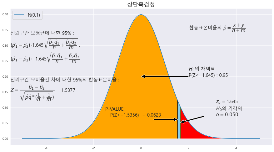
P-value = 0.0623
alpha = 0.05
귀무가설 H_0 : 도시 사람의 찬성률이 농어촌 사람의 찬성률보다 작거나 같다.
p-value > alpha ==> 0.0623 > 0.05 ==> 귀무가설 채택 ==> 도시 사람의 찬성률이 농어촌 사람의 찬성률보다 크지 않다.
26. 남학생 650명과 여학생 555명을 대상으로 학업을 위하여 아르바이트를 하고 있는지 설문 조사를 실시한 결과, 남학생 403명과 여학생 389명이 아르바이트를 하고 있는 것으로 조사되었다. 아르바이트하는 남학생의 비율이 여학생의 비율보다 낮은지 유의수준 1%에서 조사하라.
^p_1 = 403/650
^p_2 = 389/555
==> ^p_1 - ^p_2 < 0 ==> 하단측 검정
==> 표본편차 존재 x ==> 표본비율의 차에 따른 검정 시행
p1 < p2
==> H_0 : p_1 >= p_2 ==> 아르바이트 하는 남학생의 비율이 여학생의 비율보다 크거나 같다.
x = np.arange(-5,5 , .001)

fig = plt.figure(figsize=(15,8))
ax = sns.lineplot(x , stats.norm.pdf(x, loc=0 , scale =1)) #정의역 범위 , 평균 = 0 , 표준편차 =1 인 정규분포 플롯

# trust = 95 #신뢰도
p1 = 403/650
p2 = 389/555

n = 650
m = 555


ax.set_title('하단측검정' ,fontsize = 18)
RATIO = round(p1 - p2,4)
SAMPLE_PROP = (403 + 389) / (n+m) #합동표본비율

#==========================================귀무가설 기각과 채택 ====================================================
trust = 95 #신뢰도_유의수준

t_1  = round(scipy.stats.norm.ppf(1-(1-(trust/100))) ,3 )


ax.fill_between(x, stats.norm.pdf(x, loc=0 , scale =1) , 0 , where =  (x>=-t_1) , facecolor = 'orange') # x값 , y값 , 0 , x<=0 인곳 , 색깔
area = 1- scipy.stats.norm.cdf(-t_1)

plt.annotate('' , xy=(0, .2), xytext=(2 , .2)  , arrowprops = dict(facecolor = 'black'))
ax.text(2 , .2, r'$H_{0}$의 채택역' +f'\nP(Z<={-t_1}) : {round(area,4)}',fontsize=15)

annotate_len = stats.norm.pdf(t_1, loc=0 , scale =1) /2
ax.vlines(x= -t_1, ymin= 0 , ymax= stats.norm.pdf(-t_1, loc=0 , scale =1) , color = 'green' , linestyle ='solid' , label ='{}'.format(2))
# ax.vlines(x= -t_1, ymin= 0 , ymax= stats.norm.pdf(-t_1, loc=0 , scale =1) , color = 'green' , linestyle ='solid' , label ='{}'.format(2))

area = round((1-area) ,3)
# ax.text(1 + t_1 , annotate_len+0.02 , r'$z_{\alpha} = $' + f'{t_1}\n' + r'$H_{0}$의 기각역' + f'\n'+ r'$\alpha = {%.3f}$' % area,fontsize=15)
ax.text(-1.5 -t_1 , annotate_len+0.02 , r'$z_{\alpha} = $' + f'{-t_1}\n' + r'$H_{0}$의 기각역' + f'\n'+ r'$\alpha = {%.3f}$' % area,fontsize=15)


# plt.annotate('' , xy=(t_1, annotate_len), xytext=(t_1+ 1 , annotate_len+0.02)  , arrowprops = dict(facecolor = 'black'))
plt.annotate('' , xy=(-t_1, annotate_len), xytext=(-1-t_1 , annotate_len+0.02)  , arrowprops = dict(facecolor = 'black'))


ax.text(-5.5 , .25, f'신뢰구간 모평균에 대한 {trust}% : \n' + r'$\left(\widehat{p}_{1} - \widehat{p}_{2}\right)$' +f'-{t_1}' + r'$\sqrt{\dfrac{\widehat{p}_{1}\widehat{q}_{1}}{n}+\dfrac{\widehat{p}_{2}\widehat{q}_{2}}{m}}$' +' , \n'+ r'$\left(\widehat{p}_{1} - \widehat{p}_{2}\right)$' +f'+ {t_1}' + r'$\sqrt{\dfrac{\widehat{p}_{1}\widehat{q}_{1}}{n}+\dfrac{\widehat{p}_{2}\widehat{q}_{2}}{m}}$',fontsize=15)

ax.text(-5.5 , .15, f'신뢰구간 모비율간 차에 대한 {trust}%의 합동표본비율 : \n' + r'$Z = \dfrac{\widehat{p}_1 - \widehat{p}_2}{ \sqrt{\widehat{p}\widehat{q} * (\dfrac{1}{n} + \dfrac{1}{m}})  }$' + f'=  { round((p1 - p2) / math.sqrt(SAMPLE_PROP * (1-SAMPLE_PROP) * ( (1 / n) + (1/m))),4) }',fontsize=15)


# ax.text(-5.5 , .25, f'귀무가설 : 남자(u_1)의 입원일수가 여자(u_2)의 입원일수 보다 작다.\n u_1 < u_2'  , fontsize = 15)
ax.text(2 , .35 , r'합동표본비율의 $ \widehat{p} = \dfrac{x + y}{n + m}$' ,fontsize= 15)


#============================================표본평균의 정규분포화 =========================================================


STDS = math.sqrt( SAMPLE_PROP * (1-SAMPLE_PROP) * (1/n + 1/m))
# print(math.sqrt(SAMPLE_PROP * (1-SAMPLE_PROP) * (1/n + 1/m) ))
# print(RATIO)
# print(f'STDS :{STDS}' )

z_1 = round(RATIO/STDS  , 4)
# z_1 =(9.075 - 7.114) / 1.6035
# # z_2 = round((34.5 - 35) / math.sqrt(5.5**2 / 25) , 2)
# z_1 = round(scipy.stats.norm.ppf(1 - (1-(trust/100))/2) ,3 )
z_1 = abs(z_1)
print(z_1)
ax.fill_between(x, stats.norm.pdf(x, loc=0 , scale =1) , 0 , where = (x<=-z_1)  , facecolor = 'skyblue') # x값 , y값 , 0 , x<=0 인곳 , 색깔
ax.fill_between(x, stats.norm.pdf(x, loc=0 , scale =1) , 0 , where = (x<=-t_1)  , facecolor = 'red') # x값 , y값 , 0 , x<=0 인곳 , 색깔
area = scipy.stats.norm.cdf(-z_1)


ax.vlines(x= -z_1, ymin= 0 , ymax= stats.norm.pdf(z_1, loc=0 , scale =1) , color = 'black' , linestyle ='solid' , label ='{}'.format(2))
# ax.vlines(x= -z_1, ymin= 0 , ymax= stats.norm.pdf(-z_1, loc=0 , scale =1) , color = 'black' , linestyle ='solid' , label ='{}'.format(2))

annotate_len = stats.norm.pdf(z_1, loc=0 , scale =1) /2
plt.annotate('' , xy=(-z_1, annotate_len), xytext=(-z_1 +1.5 , annotate_len+0.02)  , arrowprops = dict(facecolor = 'black'))
# plt.annotate('' , xy=(-z_1, annotate_len), xytext=(1-z_1 , annotate_len)  , arrowprops = dict(facecolor = 'black'))
ax.text(-1.5 , annotate_len+0.01 , f'P-VALUE: \n   P(Z<={-z_1})  = {round(area,4)}',fontsize=15)


b= 'N(0,1)'

plt.legend([b] , fontsize = 15 , loc='upper left')
#
# print( (9.075 - 7.114) / 1.6035)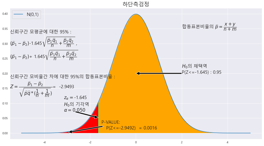
P-value = 0.0016
alpha = 0.05
귀무가설 H_0 : 남학생의 비율이 여학생보다 높거나 같다.
p-value < alpha ==> 0.0016 < 0.05 ==> 귀무가설 기각 ==> 남학생의 비율이 여학생의 비율보다 낮다.
'기초통계 > 대표본 가설검정' 카테고리의 다른 글
| ★상단/하단 구분시 찾으려는 가설의 부등호 위치에 주목하자★표본평균의 차에 대한 가설 검정★기초통계학-[연습문제 05 -13] (0) | 2023.01.16 |
|---|---|
| ★귀무가설 설정 중요!!!!!!!(부등호가 존재)★표본평균의 차에 대한 가설 검정★모평균의 차에 대한 가설 검정★기초통계학-[연습문제 04 -12] (0) | 2023.01.16 |
| ★표본비율의 정규분포화★모비율의 가설 검정★기초통계학-[연습문제 03 -11] (0) | 2023.01.16 |
| ★모평균의 가설 검정★기초통계학-[연습문제 02 -10] (1) | 2023.01.16 |
| ★=이 있는것이 귀무가설★모평균의 양측검정★모평균 <= |X 상단측 검정★모평균 >= |X 하단측검정★기초통계학-[연습문제 01 -09] (2) | 2023.01.16 |
★상단/하단 구분시 찾으려는 가설의 부등호 위치에 주목하자★표본평균의 차에 대한 가설 검정★기초통계학-[연습문제 05 -13]
20. 12세 이하의 남자아이가 여자아이에 비해 주당 TV 시청 시간이 더 많은지 알아보기 위하여 조사한 결과 다음과 같다. 이것을 근거로 남자아이가 여자아이보다 TV를 더 많이 시청하는지 유의수준 5%에서 조사하라.
A = pd.DataFrame(columns = ['표본평균' , '모표준편차' , '표본의크기'] , index = ['남자아이' , '여자아이'])
A['표본평균'] = [14.5 , 13.7 ]
A['모표준편차'] = [2.1, 2.7]
A['표본의크기'] = [48 , 42]
A
H_0 : X <= Y (상단측 검정)
대립가설 : X>Y
x = np.arange(-5,5 , .001)

fig = plt.figure(figsize=(15,8))
ax = sns.lineplot(x , stats.norm.pdf(x, loc=0 , scale =1)) #정의역 범위 , 평균 = 0 , 표준편차 =1 인 정규분포 플롯

# trust = 95 #신뢰도

MEANS_A = 14.5
MEANS_B = 13.7
MEANS = round(MEANS_A-MEANS_B ,3)
std_a = 2.1
std_b = 2.7
n_a = 48
n_b = 42
STDS = round(math.sqrt( (std_a**2/n_a) + (std_b**2/n_b)),4)


ax.set_title('상단측검정' ,fontsize = 18)


#==========================================귀무가설 기각과 채택 ====================================================
trust = 95 #신뢰도_유의수준

t_1  = round(scipy.stats.norm.ppf((trust/100)) ,3 )
print(t_1)

ax.fill_between(x, stats.norm.pdf(x, loc=0 , scale =1) , 0 , where =  (x<=t_1) , facecolor = 'orange') # x값 , y값 , 0 , x<=0 인곳 , 색깔
area = scipy.stats.norm.cdf(t_1)

plt.annotate('' , xy=(0, .2), xytext=(2 , .2)  , arrowprops = dict(facecolor = 'black'))
ax.text(2 , .2, r'$H_{0}$의 채택역' +f'\nP(Z<={t_1}) : {round(area,4)}',fontsize=15)

annotate_len = stats.norm.pdf(t_1, loc=0 , scale =1) /2
# ax.vlines(x= t_1, ymin= 0 , ymax= stats.norm.pdf(t_1, loc=0 , scale =1) , color = 'green' , linestyle ='solid' , label ='{}'.format(2))
ax.vlines(x= t_1, ymin= 0 , ymax= stats.norm.pdf(t_1, loc=0 , scale =1) , color = 'green' , linestyle ='solid' , label ='{}'.format(2))

# ax.text(1 + t_1 , annotate_len , r'$z_{\alpha/2} = $' + f'{t_1}\n' + r'$H_{0}$의 기각역',fontsize=15)
area = 1-area
ax.text(1 + t_1  , annotate_len , r'$z_{\alpha} = $' + f'{t_1}\n' + r'$H_{0}$의 기각역'+f'\n' +r'$\alpha = {%.3f}$' % area,fontsize=15)


# plt.annotate('' , xy=(t_1, annotate_len-0.02), xytext=(t_1+ 1 , annotate_len)  , arrowprops = dict(facecolor = 'black'))
plt.annotate('' , xy=(t_1, annotate_len), xytext=(t_1+ 1 , annotate_len)  , arrowprops = dict(facecolor = 'black'))

ax.text(-5.5 , .25, f'신뢰구간 모평균에 대한 {trust}% : \n' + r'$\left( \overline{x}-\overline{y}\right)$' +f'-{t_1}' + r'$\sqrt{\dfrac{\sigma_{1}^{2}}{n}+\dfrac{\sigma_{2} ^{2}}{m}}$' +' , '+ r'$\left( \overline{x}-\overline{y}\right)$' +f'+ {t_1}' + r'$\sqrt{\dfrac{\sigma_{1}^{2}}{n}+\dfrac{\sigma_{2} ^{2}}{m}}$',fontsize=15)

ax.text(-5.5 , .2 , f'표준오차 :' + r'$\sqrt{\dfrac{\sigma_{1}^{2}}{n}+\dfrac{\sigma_{2} ^{2}}{m}}$' + f'= {round(STDS,3)}' , fontsize = 15)

ax.text(-5.5 , .15,  r'오차한계 = ${%.3f}\sqrt{\dfrac{\sigma_{1}^{2}}{n}+\dfrac{\sigma_{2} ^{2}}{m}} = $' % t_1 + f'{round(t_1 * STDS , 3)}',fontsize=15)


ax.text(2 , .3,  r'$\overline{X}_{1}$ = ' +f'{MEANS_A}'+   r' , $\overline{X}_{2}$ = ' +f'{MEANS_B}\n' + r'$\sigma_{1} = $' + f'{std_a}' + r', $\sigma_{2} = $' + f'{std_b}\n' + r'$\sqrt{n} = $' + f'{round(math.sqrt(n_a),3)}' + r', $\sqrt{m} = $' + f'{round(math.sqrt(n_b),3)}\n'
        + r'Z = $\dfrac{\overline{X}_{1} - \overline{X}_{2}} {\sqrt{\dfrac{\sigma_{1}^{2}}{n} + \dfrac{\sigma_{2}^{2}}{m}}}$'
        + f'= {round(MEANS / STDS,4)}' ,fontsize=15)


#============================================표본평균의 정규분포화 =========================================================


z_1 = round(MEANS/ STDS ,4)
# # z_2 = round((34.5 - 35) / math.sqrt(5.5**2 / 25) , 2)
# z_1 = round(scipy.stats.norm.ppf(1 - (1-(trust/100))/2) ,3 )
z_1 = abs(z_1)
ax.fill_between(x, stats.norm.pdf(x, loc=0 , scale =1) , 0 , where = (x>=z_1)  , facecolor = 'skyblue') # x값 , y값 , 0 , x<=0 인곳 , 색깔
ax.fill_between(x, stats.norm.pdf(x, loc=0 , scale =1) , 0 , where =  (x>=t_1) , facecolor = 'red') # x값 , y값 , 0 , x<=0 인곳 , 색깔
area = 1- scipy.stats.norm.cdf(z_1)


ax.vlines(x= z_1, ymin= 0 , ymax= stats.norm.pdf(z_1, loc=0 , scale =1) , color = 'black' , linestyle ='solid' , label ='{}'.format(2))
# ax.vlines(x= -z_1, ymin= 0 , ymax= stats.norm.pdf(-z_1, loc=0 , scale =1) , color = 'black' , linestyle ='solid' , label ='{}'.format(2))

annotate_len = stats.norm.pdf(z_1, loc=0 , scale =1) /2
# plt.annotate('' , xy=(z_1, annotate_len), xytext=(z_1+ 1 , annotate_len)  , arrowprops = dict(facecolor = 'black'))
plt.annotate('' , xy=( z_1 ,  annotate_len), xytext=(0, annotate_len)  , arrowprops = dict(facecolor = 'black'))
ax.text(-1 , annotate_len+0.01 , f'p-value \n P(Z>={z_1})  = {round(area,4)}',fontsize=15)


b= 'N(0,1)'

plt.legend([b] , fontsize = 15 , loc='upper left')
P-value = 0.0606
alpha = 0.05
H_0 : X <= Y (상단측 검정) ==> 남자의 TV시청 시간이 여자보다 작거나 같다.
p-value > alpha ==> 0.0606 > 0.05 ==> 귀무가설 채택 ==> 남자의 TV시청 시간이 여자보다 작거나 같다.
21. 어느 패스트푸드 가게에서 근무하는 종업원 A의 서비스 시간이 종업원 B보다 긴지 알아보기 위하여 조사한 결과 다음과 같았다. 이것을 근거로 종업원 A가 종업원 B보다 서비스 시간이 긴지 유의수준 1%에서 조사하라.
A = pd.DataFrame(columns = ['표본평균' , '모표준편차' , '표본의크기'] , index = ['종업원 A' , '종업원 B'])
A['표본평균'] = [4.5 , 4.3 ]
A['모표준편차'] = [0.45, 0.42]
A['표본의크기'] = [50 ,80]
A
H_0 : M_A <= M_B (상단측 검정)
x = np.arange(-5,5 , .001)

fig = plt.figure(figsize=(15,8))
ax = sns.lineplot(x , stats.norm.pdf(x, loc=0 , scale =1)) #정의역 범위 , 평균 = 0 , 표준편차 =1 인 정규분포 플롯

# trust = 95 #신뢰도

MEANS_A = 4.5
MEANS_B = 4.3
MEANS = round(MEANS_A-MEANS_B ,3)
std_a = 0.45
std_b = 0.42
n_a = 50
n_b = 80
STDS = round(math.sqrt( (std_a**2/n_a) + (std_b**2/n_b)),4)


ax.set_title('상단측검정' ,fontsize = 18)


#==========================================귀무가설 기각과 채택 ====================================================
trust = 99 #신뢰도_유의수준

t_1  = round(scipy.stats.norm.ppf((trust/100)) ,3 )
print(t_1)

ax.fill_between(x, stats.norm.pdf(x, loc=0 , scale =1) , 0 , where =  (x<=t_1) , facecolor = 'orange') # x값 , y값 , 0 , x<=0 인곳 , 색깔
area = scipy.stats.norm.cdf(t_1)

plt.annotate('' , xy=(0, .2), xytext=(2 , .2)  , arrowprops = dict(facecolor = 'black'))
ax.text(2 , .2, r'$H_{0}$의 채택역' +f'\nP(Z<={t_1}) : {round(area,4)}',fontsize=15)

annotate_len = stats.norm.pdf(t_1, loc=0 , scale =1) /2
# ax.vlines(x= t_1, ymin= 0 , ymax= stats.norm.pdf(t_1, loc=0 , scale =1) , color = 'green' , linestyle ='solid' , label ='{}'.format(2))
ax.vlines(x= t_1, ymin= 0 , ymax= stats.norm.pdf(t_1, loc=0 , scale =1) , color = 'green' , linestyle ='solid' , label ='{}'.format(2))

# ax.text(1 + t_1 , annotate_len , r'$z_{\alpha/2} = $' + f'{t_1}\n' + r'$H_{0}$의 기각역',fontsize=15)
area = 1-area
ax.text(1 + t_1  , annotate_len , r'$z_{\alpha} = $' + f'{t_1}\n' + r'$H_{0}$의 기각역'+f'\n' +r'$\alpha = {%.3f}$' % area,fontsize=15)


# plt.annotate('' , xy=(t_1, annotate_len-0.02), xytext=(t_1+ 1 , annotate_len)  , arrowprops = dict(facecolor = 'black'))
plt.annotate('' , xy=(t_1, annotate_len), xytext=(t_1+ 1 , annotate_len)  , arrowprops = dict(facecolor = 'black'))

ax.text(-5.5 , .25, f'신뢰구간 모평균에 대한 {trust}% : \n' + r'$\left( \overline{x}-\overline{y}\right)$' +f'-{t_1}' + r'$\sqrt{\dfrac{\sigma_{1}^{2}}{n}+\dfrac{\sigma_{2} ^{2}}{m}}$' +' , '+ r'$\left( \overline{x}-\overline{y}\right)$' +f'+ {t_1}' + r'$\sqrt{\dfrac{\sigma_{1}^{2}}{n}+\dfrac{\sigma_{2} ^{2}}{m}}$',fontsize=15)

ax.text(-5.5 , .2 , f'표준오차 :' + r'$\sqrt{\dfrac{\sigma_{1}^{2}}{n}+\dfrac{\sigma_{2} ^{2}}{m}}$' + f'= {round(STDS,3)}' , fontsize = 15)

ax.text(-5.5 , .15,  r'오차한계 = ${%.3f}\sqrt{\dfrac{\sigma_{1}^{2}}{n}+\dfrac{\sigma_{2} ^{2}}{m}} = $' % t_1 + f'{round(t_1 * STDS , 3)}',fontsize=15)


ax.text(2 , .3,  r'$\overline{X}_{1}$ = ' +f'{MEANS_A}'+   r' , $\overline{X}_{2}$ = ' +f'{MEANS_B}\n' + r'$\sigma_{1} = $' + f'{std_a}' + r', $\sigma_{2} = $' + f'{std_b}\n' + r'$\sqrt{n} = $' + f'{round(math.sqrt(n_a),3)}' + r', $\sqrt{m} = $' + f'{round(math.sqrt(n_b),3)}\n'
        + r'Z = $\dfrac{\overline{X}_{1} - \overline{X}_{2}} {\sqrt{\dfrac{\sigma_{1}^{2}}{n} + \dfrac{\sigma_{2}^{2}}{m}}}$'
        + f'= {round(MEANS / STDS,4)}' ,fontsize=15)


#============================================표본평균의 정규분포화 =========================================================


z_1 = round(MEANS/ STDS ,4)
# # z_2 = round((34.5 - 35) / math.sqrt(5.5**2 / 25) , 2)
# z_1 = round(scipy.stats.norm.ppf(1 - (1-(trust/100))/2) ,3 )
z_1 = abs(z_1)
ax.fill_between(x, stats.norm.pdf(x, loc=0 , scale =1) , 0 , where = (x>=z_1)  , facecolor = 'skyblue') # x값 , y값 , 0 , x<=0 인곳 , 색깔
ax.fill_between(x, stats.norm.pdf(x, loc=0 , scale =1) , 0 , where =  (x>=t_1) , facecolor = 'red') # x값 , y값 , 0 , x<=0 인곳 , 색깔
area = 1- scipy.stats.norm.cdf(z_1)


ax.vlines(x= z_1, ymin= 0 , ymax= stats.norm.pdf(z_1, loc=0 , scale =1) , color = 'black' , linestyle ='solid' , label ='{}'.format(2))
# ax.vlines(x= -z_1, ymin= 0 , ymax= stats.norm.pdf(-z_1, loc=0 , scale =1) , color = 'black' , linestyle ='solid' , label ='{}'.format(2))

annotate_len = stats.norm.pdf(z_1, loc=0 , scale =1) /2
# plt.annotate('' , xy=(z_1, annotate_len), xytext=(z_1+ 1 , annotate_len)  , arrowprops = dict(facecolor = 'black'))
plt.annotate('' , xy=( z_1 ,  annotate_len), xytext=(0, annotate_len)  , arrowprops = dict(facecolor = 'black'))
ax.text(-1 , annotate_len+0.01 , f'p-value \n P(Z>={z_1})  = {round(area,4)}',fontsize=15)


b= 'N(0,1)'

plt.legend([b] , fontsize = 15 , loc='upper left')
P-value = 0.0057
alpha = 0.01
H_0 : M_A <= M_B (상단측 검정) ==> A의 근무시간이 B보다 작거나 같다.
p-value < alpha ==> 0.0057 < 0.01 ==> 귀무가설 기각 ==> A의 근무시간이 B보다 길다.
22. 울산 지역의 1인당 평균 소득이 서울보다 150만원 이상 더 많은지 알아보기 위하여 두 도시에 거주하는 사람을 각각 100명씩 임의로 선정하여 조사한 결과 다음 표와 같았다. 이것을 근거로 울산 지역의 평균 소득이 서울보다 150만원 이상 더 많은지 유의수준 5%에서 조사하라.
A = pd.DataFrame(columns = ['평균' , '표준편차' ] , index = ['울산' , '서울'])
A['평균'] = [1854 , 1684 ]
A['표준편차'] = [69.9, 73.3]
A
H_0 : 울산- 서울 >= 150 (상단측 검정) ==> 찾으려는 가설의 부등호 위치에 주목하자.
x = np.arange(-5,5 , .001)

fig = plt.figure(figsize=(15,8))
ax = sns.lineplot(x , stats.norm.pdf(x, loc=0 , scale =1)) #정의역 범위 , 평균 = 0 , 표준편차 =1 인 정규분포 플롯

# trust = 95 #신뢰도

MEANS_A = 1854
MEANS_B = 1684 + 150
MEANS = round(MEANS_A-MEANS_B ,3)
std_a = 69.9
std_b = 73.3
n_a = 100
n_b = 100
STDS = round(math.sqrt( (std_a**2/n_a) + (std_b**2/n_b)),4)


ax.set_title('상단측검정' ,fontsize = 18)


#==========================================귀무가설 기각과 채택 ====================================================
trust = 95 #신뢰도_유의수준

t_1  = round(scipy.stats.norm.ppf((trust/100)) ,3 )
print(t_1)

ax.fill_between(x, stats.norm.pdf(x, loc=0 , scale =1) , 0 , where =  (x<=t_1) , facecolor = 'orange') # x값 , y값 , 0 , x<=0 인곳 , 색깔
area = scipy.stats.norm.cdf(t_1)

plt.annotate('' , xy=(0, .2), xytext=(2 , .2)  , arrowprops = dict(facecolor = 'black'))
ax.text(2 , .2, r'$H_{0}$의 채택역' +f'\nP(Z<={t_1}) : {round(area,4)}',fontsize=15)

annotate_len = stats.norm.pdf(t_1, loc=0 , scale =1) /2
# ax.vlines(x= t_1, ymin= 0 , ymax= stats.norm.pdf(t_1, loc=0 , scale =1) , color = 'green' , linestyle ='solid' , label ='{}'.format(2))
ax.vlines(x= t_1, ymin= 0 , ymax= stats.norm.pdf(t_1, loc=0 , scale =1) , color = 'green' , linestyle ='solid' , label ='{}'.format(2))

# ax.text(1 + t_1 , annotate_len , r'$z_{\alpha/2} = $' + f'{t_1}\n' + r'$H_{0}$의 기각역',fontsize=15)
area = 1-area
ax.text(1 + t_1  , annotate_len , r'$z_{\alpha} = $' + f'{t_1}\n' + r'$H_{0}$의 기각역'+f'\n' +r'$\alpha = {%.3f}$' % area,fontsize=15)


# plt.annotate('' , xy=(t_1, annotate_len-0.02), xytext=(t_1+ 1 , annotate_len)  , arrowprops = dict(facecolor = 'black'))
plt.annotate('' , xy=(t_1, annotate_len), xytext=(t_1+ 1 , annotate_len)  , arrowprops = dict(facecolor = 'black'))

ax.text(-5.5 , .25, f'신뢰구간 모평균에 대한 {trust}% : \n' + r'$\left( \overline{x}-\overline{y}\right)$' +f'-{t_1}' + r'$\sqrt{\dfrac{\sigma_{1}^{2}}{n}+\dfrac{\sigma_{2} ^{2}}{m}}$' +' , '+ r'$\left( \overline{x}-\overline{y}\right)$' +f'+ {t_1}' + r'$\sqrt{\dfrac{\sigma_{1}^{2}}{n}+\dfrac{\sigma_{2} ^{2}}{m}}$',fontsize=15)

ax.text(-5.5 , .2 , f'표준오차 :' + r'$\sqrt{\dfrac{\sigma_{1}^{2}}{n}+\dfrac{\sigma_{2} ^{2}}{m}}$' + f'= {round(STDS,3)}' , fontsize = 15)

ax.text(-5.5 , .15,  r'오차한계 = ${%.3f}\sqrt{\dfrac{\sigma_{1}^{2}}{n}+\dfrac{\sigma_{2} ^{2}}{m}} = $' % t_1 + f'{round(t_1 * STDS , 3)}',fontsize=15)


ax.text(2 , .3,  r'$\overline{X}_{1}$ = ' +f'{MEANS_A}'+   r' , $\overline{X}_{2}$ = ' +f'{MEANS_B}\n' + r'$\sigma_{1} = $' + f'{std_a}' + r', $\sigma_{2} = $' + f'{std_b}\n' + r'$\sqrt{n} = $' + f'{round(math.sqrt(n_a),3)}' + r', $\sqrt{m} = $' + f'{round(math.sqrt(n_b),3)}\n'
        + r'Z = $\dfrac{\overline{X}_{1} - \overline{X}_{2}} {\sqrt{\dfrac{\sigma_{1}^{2}}{n} + \dfrac{\sigma_{2}^{2}}{m}}}$'
        + f'= {round(MEANS / STDS,4)}' ,fontsize=15)


#============================================표본평균의 정규분포화 =========================================================


z_1 = round(MEANS/ STDS ,4)
# # z_2 = round((34.5 - 35) / math.sqrt(5.5**2 / 25) , 2)
# z_1 = round(scipy.stats.norm.ppf(1 - (1-(trust/100))/2) ,3 )
z_1 = abs(z_1)
ax.fill_between(x, stats.norm.pdf(x, loc=0 , scale =1) , 0 , where = (x>=z_1)  , facecolor = 'skyblue') # x값 , y값 , 0 , x<=0 인곳 , 색깔
ax.fill_between(x, stats.norm.pdf(x, loc=0 , scale =1) , 0 , where =  (x>=t_1) , facecolor = 'red') # x값 , y값 , 0 , x<=0 인곳 , 색깔
area = 1- scipy.stats.norm.cdf(z_1)


ax.vlines(x= z_1, ymin= 0 , ymax= stats.norm.pdf(z_1, loc=0 , scale =1) , color = 'black' , linestyle ='solid' , label ='{}'.format(2))
# ax.vlines(x= -z_1, ymin= 0 , ymax= stats.norm.pdf(-z_1, loc=0 , scale =1) , color = 'black' , linestyle ='solid' , label ='{}'.format(2))

annotate_len = stats.norm.pdf(z_1, loc=0 , scale =1) /2
# plt.annotate('' , xy=(z_1, annotate_len), xytext=(z_1+ 1 , annotate_len)  , arrowprops = dict(facecolor = 'black'))
plt.annotate('' , xy=( z_1 ,  annotate_len), xytext=(0, annotate_len)  , arrowprops = dict(facecolor = 'black'))
ax.text(-1 , annotate_len+0.01 , f'p-value \n P(Z>={z_1})  = {round(area,4)}',fontsize=15)


b= 'N(0,1)'

plt.legend([b] , fontsize = 15 , loc='upper left')

P-value = 0.0242
alpha = 0.05
H_0 : 울산- 서울 >= 150 (상단측 검정) ==> 울산의 1인당 평균소득이 서울보다 150만원 이상이다.
p-value < alpha ==> 0.0242 < 0.05 ==> 귀무가설 기각 ==> 울산의 1인당 평균소득이 서울보다 150만원 미만이다.
'기초통계 > 대표본 가설검정' 카테고리의 다른 글
| ★표본비율의 차에 따른 검정★합동표본비율★표본분산 모를때는 표본비율의 차로 검정★기초통계학-[연습문제 06 -14] (0) | 2023.01.16 |
|---|---|
| ★귀무가설 설정 중요!!!!!!!(부등호가 존재)★표본평균의 차에 대한 가설 검정★모평균의 차에 대한 가설 검정★기초통계학-[연습문제 04 -12] (0) | 2023.01.16 |
| ★표본비율의 정규분포화★모비율의 가설 검정★기초통계학-[연습문제 03 -11] (0) | 2023.01.16 |
| ★모평균의 가설 검정★기초통계학-[연습문제 02 -10] (1) | 2023.01.16 |
| ★=이 있는것이 귀무가설★모평균의 양측검정★모평균 <= |X 상단측 검정★모평균 >= |X 하단측검정★기초통계학-[연습문제 01 -09] (2) | 2023.01.16 |
★귀무가설 설정 중요!!!!!!!(부등호가 존재)★표본평균의 차에 대한 가설 검정★모평균의 차에 대한 가설 검정★기초통계학-[연습문제 04 -12]
15. 두 모집단의 평균이 동일한지 알아보기 위하여 각각 크기 36인 표본을 조사하여 다음을 얻었다. 이것을 근거로 p-value 값을 구하고, 모평균이 동일한지 유의수준 5%에서 조사하라.
A = pd.DataFrame(columns = ['표본평균' , '모표준편차'] , index = ['A' , 'B'])
A['표본평균'] = [27.3 , 24.8]
A['모표준편차'] = [5.2 , 6.0]
A

x = np.arange(-5,5 , .001)

fig = plt.figure(figsize=(15,8))
ax = sns.lineplot(x , stats.norm.pdf(x, loc=0 , scale =1)) #정의역 범위 , 평균 = 0 , 표준편차 =1 인 정규분포 플롯

# trust = 95 #신뢰도

MEANS_A = 27.3
MEANS_B = 24.8
MEANS = round(MEANS_A-MEANS_B ,3)
std_a = 5.2
std_b = 6
n_a = 36
n_b = 36
STDS = round(math.sqrt( (std_a**2/n_a) + (std_b**2/n_b)),4)


ax.set_title('하단측검정' ,fontsize = 18)


#==========================================귀무가설 기각과 채택 ====================================================
trust = 95 #신뢰도_유의수준

t_1  = round(scipy.stats.norm.ppf((trust/100)) ,3 )
print(t_1)

ax.fill_between(x, stats.norm.pdf(x, loc=0 , scale =1) , 0 , where =  (x>=-t_1) , facecolor = 'orange') # x값 , y값 , 0 , x<=0 인곳 , 색깔
area = scipy.stats.norm.cdf(t_1)

plt.annotate('' , xy=(0, .2), xytext=(2 , .2)  , arrowprops = dict(facecolor = 'black'))
ax.text(2 , .2, r'$H_{0}$의 채택역' +f'\nP(Z>={-t_1}) : {round(area,4)}',fontsize=15)

annotate_len = stats.norm.pdf(t_1, loc=0 , scale =1) /2
# ax.vlines(x= t_1, ymin= 0 , ymax= stats.norm.pdf(t_1, loc=0 , scale =1) , color = 'green' , linestyle ='solid' , label ='{}'.format(2))
ax.vlines(x= -t_1, ymin= 0 , ymax= stats.norm.pdf(-t_1, loc=0 , scale =1) , color = 'green' , linestyle ='solid' , label ='{}'.format(2))

# ax.text(1 + t_1 , annotate_len , r'$z_{\alpha/2} = $' + f'{t_1}\n' + r'$H_{0}$의 기각역',fontsize=15)
area = 1-area
ax.text(-2.5 -t_1 , annotate_len , r'$z_{\alpha} = $' + f'{-t_1}\n' + r'$H_{0}$의 기각역'+f'\n' +r'$\alpha = {%.3f}$' % area,fontsize=15)


# plt.annotate('' , xy=(t_1, annotate_len-0.02), xytext=(t_1+ 1 , annotate_len)  , arrowprops = dict(facecolor = 'black'))
plt.annotate('' , xy=(-t_1, annotate_len), xytext=(-1-t_1 , annotate_len)  , arrowprops = dict(facecolor = 'black'))

ax.text(-5.5 , .25, f'신뢰구간 모평균에 대한 {trust}% : \n' + r'$\left( \overline{x}-\overline{y}\right)$' +f'-{t_1}' + r'$\sqrt{\dfrac{\sigma_{1}^{2}}{n}+\dfrac{\sigma_{2} ^{2}}{m}}$' +' , '+ r'$\left( \overline{x}-\overline{y}\right)$' +f'+ {t_1}' + r'$\sqrt{\dfrac{\sigma_{1}^{2}}{n}+\dfrac{\sigma_{2} ^{2}}{m}}$',fontsize=15)

ax.text(-5.5 , .2 , f'표준오차 :' + r'$\sqrt{\dfrac{\sigma_{1}^{2}}{n}+\dfrac{\sigma_{2} ^{2}}{m}}$' + f'= {round(STDS,3)}' , fontsize = 15)

ax.text(-5.5 , .15,  r'오차한계 = ${%.3f}\sqrt{\dfrac{\sigma_{1}^{2}}{n}+\dfrac{\sigma_{2} ^{2}}{m}} = $' % t_1 + f'{round(t_1 * STDS , 3)}',fontsize=15)


ax.text(2 , .35,  r'$\overline{X}_{1}$ = ' +f'{MEANS_A}'+   r' , $\overline{X}_{2}$ = ' +f'{MEANS_B}\n' + r'$\sigma_{1} = $' + f'{std_a}' + r', $\sigma_{2} = $' + f'{std_b}\n' + r'$\sqrt{n} = $' + f'{round(math.sqrt(n_a),3)}' + r', $\sqrt{m} = $' + f'{round(math.sqrt(n_b),3)}',fontsize=15)


#============================================표본평균의 정규분포화 =========================================================


z_1 = round(MEANS/ STDS ,2)
# # z_2 = round((34.5 - 35) / math.sqrt(5.5**2 / 25) , 2)
# z_1 = round(scipy.stats.norm.ppf(1 - (1-(trust/100))/2) ,3 )
z_1 = abs(z_1)
ax.fill_between(x, stats.norm.pdf(x, loc=0 , scale =1) , 0 , where = (x<=-z_1)  , facecolor = 'skyblue') # x값 , y값 , 0 , x<=0 인곳 , 색깔
ax.fill_between(x, stats.norm.pdf(x, loc=0 , scale =1) , 0 , where =  (x<=-t_1) , facecolor = 'red') # x값 , y값 , 0 , x<=0 인곳 , 색깔
area = scipy.stats.norm.cdf(-z_1)


ax.vlines(x= -z_1, ymin= 0 , ymax= stats.norm.pdf(z_1, loc=0 , scale =1) , color = 'black' , linestyle ='solid' , label ='{}'.format(2))
# ax.vlines(x= -z_1, ymin= 0 , ymax= stats.norm.pdf(-z_1, loc=0 , scale =1) , color = 'black' , linestyle ='solid' , label ='{}'.format(2))

annotate_len = stats.norm.pdf(z_1, loc=0 , scale =1) /2
# plt.annotate('' , xy=(z_1, annotate_len), xytext=(z_1+ 1 , annotate_len)  , arrowprops = dict(facecolor = 'black'))
plt.annotate('' , xy=( -z_1 ,  annotate_len), xytext=(z_1-0.05, annotate_len)  , arrowprops = dict(facecolor = 'black'))
ax.text(-.09 , annotate_len+0.01 , f'p-value \n P(Z<={-z_1})  = {round(area,4)}',fontsize=15)
# ax.text(0 , annotate_len+0.01 ,f'P(Z>={-z_1})',fontsize=15)


#
# ax.text(2 , .35,  r'$\overline{X}$ = ' +f'{MEANS}\n'+ r'$\sigma = $' + f'{STDS}\n' + r'$\sqrt{n} = $' + f'{STDS,3)}',fontsize=15)

b= 'N(0,1)'

plt.legend([b] , fontsize = 15 , loc='upper left')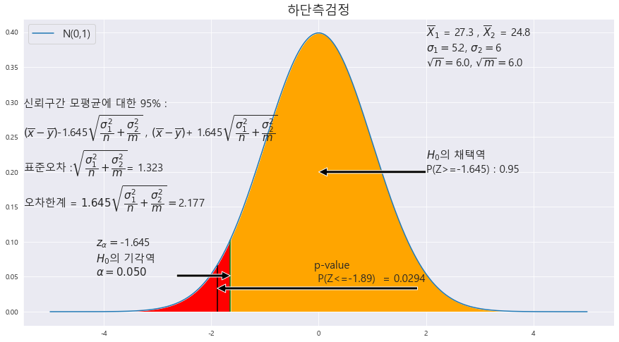
P-VALUE = 0.0294
alpha = 0.05
귀무가설 H_0 : p1 = p2 ==> ^p1 의 표본평균이 크다. ==> (하단측검정)
P-VALUE < alpha ==> 0.0294 < 0.05 ==> 귀무가설 H_0 기각 ==> 모평균이 동일하지 않다.
========================================================================================
x = np.arange(-5,5 , .001)

fig = plt.figure(figsize=(15,8))
ax = sns.lineplot(x , stats.norm.pdf(x, loc=0 , scale =1)) #정의역 범위 , 평균 = 0 , 표준편차 =1 인 정규분포 플롯

# trust = 95 #신뢰도

MEANS_A = 27.3
MEANS_B = 24.8
MEANS = round(MEANS_A-MEANS_B ,3)
std_a = 5.2
std_b = 6
n_a = 36
n_b = 36
STDS = round(math.sqrt( (std_a**2/n_a) + (std_b**2/n_b)),4)


ax.set_title('양측검정' ,fontsize = 18)


#==========================================귀무가설 기각과 채택 ====================================================
trust = 95 #신뢰도_유의수준
# trust = trust - (100-trust)
t_1  = round(scipy.stats.norm.ppf(1 - (1-(trust/100))/2) ,3 )
print(t_1)

ax.fill_between(x, stats.norm.pdf(x, loc=0 , scale =1) , 0 , where =  (x>=-t_1)  , facecolor = 'orange') # x값 , y값 , 0 , x<=0 인곳 , 색깔
area = scipy.stats.norm.cdf(t_1) - scipy.stats.norm.cdf(-t_1)

plt.annotate('' , xy=(0, .2), xytext=(2 , .2)  , arrowprops = dict(facecolor = 'black'))
ax.text(2 , .2, r'$H_{0}$의 채택역' +f'\nP({-t_1}<=Z<={t_1}) : {round(area,4)}',fontsize=15)

annotate_len = stats.norm.pdf(t_1, loc=0 , scale =1) /2
ax.vlines(x= t_1, ymin= 0 , ymax= stats.norm.pdf(t_1, loc=0 , scale =1) , color = 'green' , linestyle ='solid' , label ='{}'.format(2))
ax.vlines(x= -t_1, ymin= 0 , ymax= stats.norm.pdf(-t_1, loc=0 , scale =1) , color = 'green' , linestyle ='solid' , label ='{}'.format(2))


area = round( (1-area) / 2 , 3)
ax.text(1 + t_1 , annotate_len , r'$z_{\alpha/2} = $' + f'{t_1}\n' + r'$H_{0}$의 기각역'+f'\n' +r'$\alpha/2 = {%.3f}$' % area,fontsize=15)

ax.text(-2.5 -t_1 , annotate_len , r'$z_{\alpha/2} = $' + f'{-t_1}\n' + r'$H_{0}$의 기각역'+f'\n' +r'$\alpha/2 = {%.3f}$' % area,fontsize=15)


plt.annotate('' , xy=(t_1, annotate_len-0.02), xytext=(t_1+ 1 , annotate_len)  , arrowprops = dict(facecolor = 'black'))
plt.annotate('' , xy=(-t_1, annotate_len), xytext=(-1-t_1 , annotate_len)  , arrowprops = dict(facecolor = 'black'))


ax.text(-5.5 , .25, f'신뢰구간 모평균에 대한 {trust}% : \n' + r'$\left( \overline{x}-\overline{y}\right)$' +f'-{t_1}' + r'$\sqrt{\dfrac{\sigma_{1}^{2}}{n}+\dfrac{\sigma_{2} ^{2}}{m}}$' +' , '+ r'$\left( \overline{x}-\overline{y}\right)$' +f'+ {t_1}' + r'$\sqrt{\dfrac{\sigma_{1}^{2}}{n}+\dfrac{\sigma_{2} ^{2}}{m}}$',fontsize=15)

ax.text(-5.5 , .2 , f'표준오차 :' + r'$\sqrt{\dfrac{\sigma_{1}^{2}}{n}+\dfrac{\sigma_{2} ^{2}}{m}}$' + f'= {round(STDS,3)}' , fontsize = 15)

ax.text(-5.5 , .15,  r'오차한계 = ${%.3f}\sqrt{\dfrac{\sigma_{1}^{2}}{n}+\dfrac{\sigma_{2} ^{2}}{m}} = $' % t_1 + f'{round(t_1 * STDS , 3)}',fontsize=15)


ax.text(2 , .35,  r'$\overline{X}_{1}$ = ' +f'{MEANS_A}'+   r' , $\overline{X}_{2}$ = ' +f'{MEANS_B}\n' + r'$\sigma_{1} = $' + f'{std_a}' + r', $\sigma_{2} = $' + f'{std_b}\n' + r'$\sqrt{n} = $' + f'{round(math.sqrt(n_a),3)}' + r', $\sqrt{m} = $' + f'{round(math.sqrt(n_b),3)}',fontsize=15)


#============================================표본평균의 정규분포화 =========================================================


z_1 = round(MEANS/ STDS ,2)
# # z_2 = round((34.5 - 35) / math.sqrt(5.5**2 / 25) , 2)
# z_1 = round(scipy.stats.norm.ppf(1 - (1-(trust/100))/2) ,3 )
print(z_1)
z_1 = abs(z_1)
ax.fill_between(x, stats.norm.pdf(x, loc=0 , scale =1) , 0 , where = (x<=-z_1) | (x>=z_1)  , facecolor = 'skyblue') # x값 , y값 , 0 , x<=0 인곳 , 색깔
ax.fill_between(x, stats.norm.pdf(x, loc=0 , scale =1) , 0 , where =  (x<=-t_1) | (x>=t_1) , facecolor = 'red') # x값 , y값 , 0 , x<=0 인곳 , 색깔
area = scipy.stats.norm.cdf(-z_1) +1- scipy.stats.norm.cdf(z_1)


ax.vlines(x= z_1, ymin= 0 , ymax= stats.norm.pdf(z_1, loc=0 , scale =1) , color = 'black' , linestyle ='solid' , label ='{}'.format(2))
ax.vlines(x= -z_1, ymin= 0 , ymax= stats.norm.pdf(-z_1, loc=0 , scale =1) , color = 'black' , linestyle ='solid' , label ='{}'.format(2))

annotate_len = stats.norm.pdf(z_1, loc=0 , scale =1) /2
plt.annotate('' , xy=(z_1, annotate_len), xytext=(z_1- 1 , annotate_len)  , arrowprops = dict(facecolor = 'black'))
plt.annotate('' , xy=(-z_1, annotate_len), xytext=(1-z_1 , annotate_len)  , arrowprops = dict(facecolor = 'black'))
ax.text(-1.5 , annotate_len+0.01 , f'P-value : \nP(Z<={-z_1}) + P(Z>={z_1})  = {round(area,4)}',fontsize=15)


b= 'N(0,1)'

plt.legend([b] , fontsize = 15 , loc='upper left')

print(t_1)
==> 동일한거여서 양측 검정이 맞지 않을까?
P-VALUE = 0.0588
alpha = 0.05
귀무가설 H_0 : p1 = p2 ==>양측검정
P-VALUE > alpha ==> 0.0588 > 0.05 ==> 귀무가설 H_0 채택 ==> 모평균이 동일하다.
16. 사회계열과 공학계열 대졸 출신의 평균 임금이 동일한지 알아보기 위하여 각각 크기 50인 표본을 조사하여 다음을 얻었다. 이것을 근거로 두계열 출신의 평균 임금이 동일한지 유의수준 5%에서 조사하라.
A = pd.DataFrame(columns = ['표본평균' , '모표준편차'] , index = ['사회계열' , '공학계열'])
A['표본평균'] = [301.5 , 317.1 ]
A['모표준편차'] = [ 38.6, 43.3]
A
H_0 = 사회계열= 공학계열 (양측 검정)
x = np.arange(-5,5 , .001)

fig = plt.figure(figsize=(15,8))
ax = sns.lineplot(x , stats.norm.pdf(x, loc=0 , scale =1)) #정의역 범위 , 평균 = 0 , 표준편차 =1 인 정규분포 플롯

# trust = 95 #신뢰도

MEANS_A = 301.5
MEANS_B = 317.1
MEANS = round(MEANS_A-MEANS_B ,3)
std_a = 38.6
std_b = 43.3
n_a = 50
n_b = 50
STDS = round(math.sqrt( (std_a**2/n_a) + (std_b**2/n_b)),4)


ax.set_title('양측검정' ,fontsize = 18)


#==========================================귀무가설 기각과 채택 ====================================================
trust = 95 #신뢰도_유의수준
# trust = trust - (100-trust)
t_1  = round(scipy.stats.norm.ppf(1 - (1-(trust/100))/2) ,3 )
print(t_1)

ax.fill_between(x, stats.norm.pdf(x, loc=0 , scale =1) , 0 , where =  (x>=-t_1)  , facecolor = 'orange') # x값 , y값 , 0 , x<=0 인곳 , 색깔
area = scipy.stats.norm.cdf(t_1) - scipy.stats.norm.cdf(-t_1)

plt.annotate('' , xy=(0, .2), xytext=(2 , .2)  , arrowprops = dict(facecolor = 'black'))
ax.text(2 , .2, r'$H_{0}$의 채택역' +f'\nP({-t_1}<=Z<={t_1}) : {round(area,4)}',fontsize=15)

annotate_len = stats.norm.pdf(t_1, loc=0 , scale =1) /2
ax.vlines(x= t_1, ymin= 0 , ymax= stats.norm.pdf(t_1, loc=0 , scale =1) , color = 'green' , linestyle ='solid' , label ='{}'.format(2))
ax.vlines(x= -t_1, ymin= 0 , ymax= stats.norm.pdf(-t_1, loc=0 , scale =1) , color = 'green' , linestyle ='solid' , label ='{}'.format(2))


area = round( (1-area) / 2 , 3)
ax.text(1 + t_1 , annotate_len , r'$z_{\alpha/2} = $' + f'{t_1}\n' + r'$H_{0}$의 기각역'+f'\n' +r'$\alpha/2 = {%.3f}$' % area,fontsize=15)

ax.text(-2.5 -t_1 , annotate_len , r'$z_{\alpha/2} = $' + f'{-t_1}\n' + r'$H_{0}$의 기각역'+f'\n' +r'$\alpha/2 = {%.3f}$' % area,fontsize=15)


plt.annotate('' , xy=(t_1, annotate_len-0.02), xytext=(t_1+ 1 , annotate_len)  , arrowprops = dict(facecolor = 'black'))
plt.annotate('' , xy=(-t_1, annotate_len), xytext=(-1-t_1 , annotate_len)  , arrowprops = dict(facecolor = 'black'))


ax.text(-5.5 , .25, f'신뢰구간 모평균에 대한 {trust}% : \n' + r'$\left( \overline{x}-\overline{y}\right)$' +f'-{t_1}' + r'$\sqrt{\dfrac{\sigma_{1}^{2}}{n}+\dfrac{\sigma_{2} ^{2}}{m}}$' +' , '+ r'$\left( \overline{x}-\overline{y}\right)$' +f'+ {t_1}' + r'$\sqrt{\dfrac{\sigma_{1}^{2}}{n}+\dfrac{\sigma_{2} ^{2}}{m}}$',fontsize=15)

ax.text(-5.5 , .2 , f'표준오차 :' + r'$\sqrt{\dfrac{\sigma_{1}^{2}}{n}+\dfrac{\sigma_{2} ^{2}}{m}}$' + f'= {round(STDS,3)}' , fontsize = 15)

ax.text(-5.5 , .15,  r'오차한계 = ${%.3f}\sqrt{\dfrac{\sigma_{1}^{2}}{n}+\dfrac{\sigma_{2} ^{2}}{m}} = $' % t_1 + f'{round(t_1 * STDS , 3)}',fontsize=15)


ax.text(2 , .35,  r'$\overline{X}_{1}$ = ' +f'{MEANS_A}'+   r' , $\overline{X}_{2}$ = ' +f'{MEANS_B}\n' + r'$\sigma_{1} = $' + f'{std_a}' + r', $\sigma_{2} = $' + f'{std_b}\n' + r'$\sqrt{n} = $' + f'{round(math.sqrt(n_a),3)}' + r', $\sqrt{m} = $' + f'{round(math.sqrt(n_b),3)}',fontsize=15)


#============================================표본평균의 정규분포화 =========================================================


z_1 = round(MEANS/ STDS ,2)
# # z_2 = round((34.5 - 35) / math.sqrt(5.5**2 / 25) , 2)
# z_1 = round(scipy.stats.norm.ppf(1 - (1-(trust/100))/2) ,3 )
print(z_1)
z_1 = abs(z_1)
ax.fill_between(x, stats.norm.pdf(x, loc=0 , scale =1) , 0 , where = (x<=-z_1) | (x>=z_1)  , facecolor = 'skyblue') # x값 , y값 , 0 , x<=0 인곳 , 색깔
ax.fill_between(x, stats.norm.pdf(x, loc=0 , scale =1) , 0 , where =  (x<=-t_1) | (x>=t_1) , facecolor = 'red') # x값 , y값 , 0 , x<=0 인곳 , 색깔
area = scipy.stats.norm.cdf(-z_1) +1- scipy.stats.norm.cdf(z_1)


ax.vlines(x= z_1, ymin= 0 , ymax= stats.norm.pdf(z_1, loc=0 , scale =1) , color = 'black' , linestyle ='solid' , label ='{}'.format(2))
ax.vlines(x= -z_1, ymin= 0 , ymax= stats.norm.pdf(-z_1, loc=0 , scale =1) , color = 'black' , linestyle ='solid' , label ='{}'.format(2))

annotate_len = stats.norm.pdf(z_1, loc=0 , scale =1) /2
plt.annotate('' , xy=(z_1, annotate_len), xytext=(z_1- 1 , annotate_len)  , arrowprops = dict(facecolor = 'black'))
plt.annotate('' , xy=(-z_1, annotate_len), xytext=(1-z_1 , annotate_len)  , arrowprops = dict(facecolor = 'black'))
ax.text(-1.5 , annotate_len+0.01 , f'P-value : \nP(Z<={-z_1}) + P(Z>={z_1})  = {round(area,4)}',fontsize=15)


b= 'N(0,1)'

plt.legend([b] , fontsize = 15 , loc='upper left')

print(t_1)
귀무가설 H_0: 사회계열과 공학계열 대졸 출신의 평균 임금의 동일 여부( 사회계열 표본평균 = 공학계열 표본평균)==> 상단측 검정
p-value : 0.0574
alpha : 0.05
p-value > alpha ==> 0.0574 > 0.05 ==> 귀무가설 H_0 채택 ==> 사회계열과 공학계열 대졸 출신의 평균 임금은 동일하다.
17. 감기에 걸렸을 때 비타민 C의 효능을 알아보기 위하여, 비타민 C를 복용한 그룹과 복용하지 않은 그룹으로 나누어 회복기간을 조사하여 다음 결과를 얻었다. 이를 근거로 감기에 걸렸을 때 비타민 C가 효력이 있는지 유의수준 5%에서 조사하라.
https://knowallworld.tistory.com/307
★두 표본평균의 차에 대한 표본분포(모분산 알때 , 동일할때)★중심극한정리 활용★이표본의
1. 이표본의 표본분포 ==>지금까지는 단일 모집단의 표본에 대한 통계량의 표본분포 EX) 수능에서 남학생, 여학생 집단의 평균이 동일한지 여부 비교 ==> 비교위해서는 각각 표본을 추출하여야 한
knowallworld.tistory.com
==> 표본평균의 차에 대한 표본분포

A = pd.DataFrame(columns = ['표본평균' , '표본표준편차' , '표본의 크기'] , index = ['비타민 C를 복용한 그룹' , '비타민 C를 복용 안한 그룹'])
A['표본평균'] = [5.2 , 5.8 ]
A['표본표준편차'] = [ 1.4, 2.2]
A['표본의 크기'] = [100 , 65]
A
|X = 5.2
|Y = 5.8
귀무가설 H_0 : 비타민 C 복용 후 회복기간 >= 복용 X (하단측 검정)
대립가설 H_0 : 비타민 C 복용후 회복기간 < 복용 X
귀무가설 : 비타민 C를 복용했을 때 복용 안했을 때보다 길다.
x = np.arange(-5,5 , .001)

fig = plt.figure(figsize=(15,8))
ax = sns.lineplot(x , stats.norm.pdf(x, loc=0 , scale =1)) #정의역 범위 , 평균 = 0 , 표준편차 =1 인 정규분포 플롯

# trust = 95 #신뢰도

MEANS_A = 5.2
MEANS_B = 5.8
MEANS = round(MEANS_A-MEANS_B ,3)
std_a = 1.4
std_b = 2.2
n_a = 100
n_b = 65
STDS = round(math.sqrt( (std_a**2/n_a) + (std_b**2/n_b)),4)


ax.set_title('하단측검정' ,fontsize = 18)


#==========================================귀무가설 기각과 채택 ====================================================
trust = 95 #신뢰도_유의수준

t_1  = round(scipy.stats.norm.ppf((trust/100)) ,3 )
print(t_1)

ax.fill_between(x, stats.norm.pdf(x, loc=0 , scale =1) , 0 , where =  (x>=-t_1) , facecolor = 'orange') # x값 , y값 , 0 , x<=0 인곳 , 색깔
area = scipy.stats.norm.cdf(t_1)

plt.annotate('' , xy=(0, .2), xytext=(2 , .2)  , arrowprops = dict(facecolor = 'black'))
ax.text(2 , .2, r'$H_{0}$의 채택역' +f'\nP(Z>={-t_1}) : {round(area,4)}',fontsize=15)

annotate_len = stats.norm.pdf(t_1, loc=0 , scale =1) /2
# ax.vlines(x= t_1, ymin= 0 , ymax= stats.norm.pdf(t_1, loc=0 , scale =1) , color = 'green' , linestyle ='solid' , label ='{}'.format(2))
ax.vlines(x= -t_1, ymin= 0 , ymax= stats.norm.pdf(-t_1, loc=0 , scale =1) , color = 'green' , linestyle ='solid' , label ='{}'.format(2))

# ax.text(1 + t_1 , annotate_len , r'$z_{\alpha/2} = $' + f'{t_1}\n' + r'$H_{0}$의 기각역',fontsize=15)
area = 1-area
ax.text(-2.5 -t_1 , annotate_len , r'$z_{\alpha} = $' + f'{-t_1}\n' + r'$H_{0}$의 기각역'+f'\n' +r'$\alpha = {%.3f}$' % area,fontsize=15)


# plt.annotate('' , xy=(t_1, annotate_len-0.02), xytext=(t_1+ 1 , annotate_len)  , arrowprops = dict(facecolor = 'black'))
plt.annotate('' , xy=(-t_1, annotate_len), xytext=(-1-t_1 , annotate_len)  , arrowprops = dict(facecolor = 'black'))

ax.text(-5.5 , .25, f'신뢰구간 모평균에 대한 {trust}% : \n' + r'$\left( \overline{x}-\overline{y}\right)$' +f'-{t_1}' + r'$\sqrt{\dfrac{\sigma_{1}^{2}}{n}+\dfrac{\sigma_{2} ^{2}}{m}}$' +' , '+ r'$\left( \overline{x}-\overline{y}\right)$' +f'+ {t_1}' + r'$\sqrt{\dfrac{\sigma_{1}^{2}}{n}+\dfrac{\sigma_{2} ^{2}}{m}}$',fontsize=15)

ax.text(-5.5 , .2 , f'표준오차 :' + r'$\sqrt{\dfrac{\sigma_{1}^{2}}{n}+\dfrac{\sigma_{2} ^{2}}{m}}$' + f'= {round(STDS,3)}' , fontsize = 15)

ax.text(-5.5 , .15,  r'오차한계 = ${%.3f}\sqrt{\dfrac{\sigma_{1}^{2}}{n}+\dfrac{\sigma_{2} ^{2}}{m}} = $' % t_1 + f'{round(t_1 * STDS , 3)}',fontsize=15)


ax.text(2 , .3,  r'$\overline{X}_{1}$ = ' +f'{MEANS_A}'+   r' , $\overline{X}_{2}$ = ' +f'{MEANS_B}\n' + r'$\sigma_{1} = $' + f'{std_a}' + r', $\sigma_{2} = $' + f'{std_b}\n' + r'$\sqrt{n} = $' + f'{round(math.sqrt(n_a),3)}' + r', $\sqrt{m} = $' + f'{round(math.sqrt(n_b),3)}\n'
        + r'Z = $\dfrac{\overline{X}_{1} - \overline{X}_{2}} {\sqrt{\dfrac{\sigma_{1}^{2}}{n} + \dfrac{\sigma_{2}^{2}}{m}}}$'
        + f'= {round(MEANS / STDS,4)}' ,fontsize=15)


#============================================표본평균의 정규분포화 =========================================================


z_1 = round(MEANS/ STDS ,2)
# # z_2 = round((34.5 - 35) / math.sqrt(5.5**2 / 25) , 2)
# z_1 = round(scipy.stats.norm.ppf(1 - (1-(trust/100))/2) ,3 )
z_1 = abs(z_1)
ax.fill_between(x, stats.norm.pdf(x, loc=0 , scale =1) , 0 , where = (x<=-z_1)  , facecolor = 'skyblue') # x값 , y값 , 0 , x<=0 인곳 , 색깔
ax.fill_between(x, stats.norm.pdf(x, loc=0 , scale =1) , 0 , where =  (x<=-t_1) , facecolor = 'red') # x값 , y값 , 0 , x<=0 인곳 , 색깔
area = scipy.stats.norm.cdf(-z_1)


ax.vlines(x= -z_1, ymin= 0 , ymax= stats.norm.pdf(z_1, loc=0 , scale =1) , color = 'black' , linestyle ='solid' , label ='{}'.format(2))
# ax.vlines(x= -z_1, ymin= 0 , ymax= stats.norm.pdf(-z_1, loc=0 , scale =1) , color = 'black' , linestyle ='solid' , label ='{}'.format(2))

annotate_len = stats.norm.pdf(z_1, loc=0 , scale =1) /2
# plt.annotate('' , xy=(z_1, annotate_len), xytext=(z_1+ 1 , annotate_len)  , arrowprops = dict(facecolor = 'black'))
plt.annotate('' , xy=( -z_1 ,  annotate_len), xytext=(z_1-0.05, annotate_len)  , arrowprops = dict(facecolor = 'black'))
ax.text(-.09 , annotate_len+0.01 , f'p-value \n P(Z<={-z_1})  = {round(area,4)}',fontsize=15)
# ax.text(0 , annotate_len+0.01 ,f'P(Z>={-z_1})',fontsize=15)


#
# ax.text(2 , .35,  r'$\overline{X}$ = ' +f'{MEANS}\n'+ r'$\sigma = $' + f'{STDS}\n' + r'$\sqrt{n} = $' + f'{STDS,3)}',fontsize=15)

b= 'N(0,1)'

plt.legend([b] , fontsize = 15 , loc='upper left')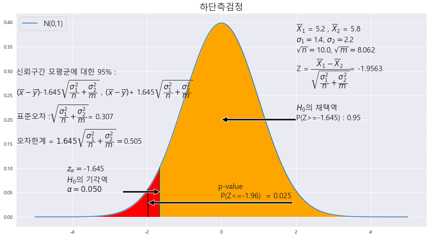
P-value = 0.0252
alpha = 0.05
귀무가설 H_0 : 비타민 C 복용 후 회복기간 >= 복용 X (하단측 검정)
p-value < alpha ==> 0.025 < 0.05 ==> 귀무가설 기각 ==> 대립가설 : 비타민 C 복용 후 회복기간 < 복용 X 후 회복기간 선정 ==> 비타민C의 복용 효과는 있다.
18. 두 그룹 A와 B의 모평균이 동일한지 알아보기 위하여 표본조사한 결과, 다음과 같았다. 이것을 근거로 모평균이 동일한지 유의수준 5%에서 조사하라.
A = pd.DataFrame(columns = ['표본평균' , '표본표준편차' , '표본의 크기'] , index = ['A' , 'B'])
A['표본평균'] = [201 , 199 ]
A['표본표준편차'] = [ 5, 6]
A['표본의 크기'] = [65 , 96]
A
H_0 : M_A = M_B(양측검정)
x = np.arange(-5,5 , .001)

fig = plt.figure(figsize=(15,8))
ax = sns.lineplot(x , stats.norm.pdf(x, loc=0 , scale =1)) #정의역 범위 , 평균 = 0 , 표준편차 =1 인 정규분포 플롯

# trust = 95 #신뢰도

MEANS_A = 201
MEANS_B = 199
MEANS = round(MEANS_A-MEANS_B ,3)
std_a = 5
std_b = 6
n_a = 65
n_b = 96
STDS = round(math.sqrt( (std_a**2/n_a) + (std_b**2/n_b)),4)


ax.set_title('양측검정' ,fontsize = 18)


#==========================================귀무가설 기각과 채택 ====================================================
trust = 95 #신뢰도_유의수준
# trust = trust - (100-trust)
t_1  = round(scipy.stats.norm.ppf(1 - (1-(trust/100))/2) ,3 )
print(t_1)

ax.fill_between(x, stats.norm.pdf(x, loc=0 , scale =1) , 0 , where =  (x>=-t_1)  , facecolor = 'orange') # x값 , y값 , 0 , x<=0 인곳 , 색깔
area = scipy.stats.norm.cdf(t_1) - scipy.stats.norm.cdf(-t_1)

plt.annotate('' , xy=(0, .2), xytext=(2 , .2)  , arrowprops = dict(facecolor = 'black'))
ax.text(2 , .2, r'$H_{0}$의 채택역' +f'\nP({-t_1}<=Z<={t_1}) : {round(area,4)}',fontsize=15)

annotate_len = stats.norm.pdf(t_1, loc=0 , scale =1) /2
ax.vlines(x= t_1, ymin= 0 , ymax= stats.norm.pdf(t_1, loc=0 , scale =1) , color = 'green' , linestyle ='solid' , label ='{}'.format(2))
ax.vlines(x= -t_1, ymin= 0 , ymax= stats.norm.pdf(-t_1, loc=0 , scale =1) , color = 'green' , linestyle ='solid' , label ='{}'.format(2))


area = round( (1-area) / 2 , 3)
ax.text(1 + t_1 , annotate_len , r'$z_{\alpha/2} = $' + f'{t_1}\n' + r'$H_{0}$의 기각역'+f'\n' +r'$\alpha/2 = {%.3f}$' % area,fontsize=15)

ax.text(-2.5 -t_1 , annotate_len , r'$z_{\alpha/2} = $' + f'{-t_1}\n' + r'$H_{0}$의 기각역'+f'\n' +r'$\alpha/2 = {%.3f}$' % area,fontsize=15)


plt.annotate('' , xy=(t_1, annotate_len-0.02), xytext=(t_1+ 1 , annotate_len)  , arrowprops = dict(facecolor = 'black'))
plt.annotate('' , xy=(-t_1, annotate_len), xytext=(-1-t_1 , annotate_len)  , arrowprops = dict(facecolor = 'black'))


ax.text(-5.5 , .25, f'신뢰구간 모평균에 대한 {trust}% : \n' + r'$\left( \overline{x}-\overline{y}\right)$' +f'-{t_1}' + r'$\sqrt{\dfrac{\sigma_{1}^{2}}{n}+\dfrac{\sigma_{2} ^{2}}{m}}$' +' , '+ r'$\left( \overline{x}-\overline{y}\right)$' +f'+ {t_1}' + r'$\sqrt{\dfrac{\sigma_{1}^{2}}{n}+\dfrac{\sigma_{2} ^{2}}{m}}$',fontsize=15)

ax.text(-5.5 , .2 , f'표준오차 :' + r'$\sqrt{\dfrac{\sigma_{1}^{2}}{n}+\dfrac{\sigma_{2} ^{2}}{m}}$' + f'= {round(STDS,3)}' , fontsize = 15)

ax.text(-5.5 , .15,  r'오차한계 = ${%.3f}\sqrt{\dfrac{\sigma_{1}^{2}}{n}+\dfrac{\sigma_{2} ^{2}}{m}} = $' % t_1 + f'{round(t_1 * STDS , 3)}',fontsize=15)


ax.text(2 , .3,  r'$\overline{X}_{1}$ = ' +f'{MEANS_A}'+   r' , $\overline{X}_{2}$ = ' +f'{MEANS_B}\n' + r'$\sigma_{1} = $' + f'{std_a}' + r', $\sigma_{2} = $' + f'{std_b}\n' + r'$\sqrt{n} = $' + f'{round(math.sqrt(n_a),3)}' + r', $\sqrt{m} = $' + f'{round(math.sqrt(n_b),3)}' + f'\n' + r'Z = $\dfrac{\overline{X}_{1} - \overline{X}_{2}} {\sqrt{\dfrac{\sigma_{1}^{2}}{n} + \dfrac{\sigma_{2}^{2}}{m}}}$'
        + f'= {round(MEANS / STDS,4)}',fontsize=15)


#============================================표본평균의 정규분포화 =========================================================


z_1 = round(MEANS/ STDS ,2)
# # z_2 = round((34.5 - 35) / math.sqrt(5.5**2 / 25) , 2)
# z_1 = round(scipy.stats.norm.ppf(1 - (1-(trust/100))/2) ,3 )
print(z_1)
z_1 = abs(z_1)
ax.fill_between(x, stats.norm.pdf(x, loc=0 , scale =1) , 0 , where = (x<=-z_1) | (x>=z_1)  , facecolor = 'skyblue') # x값 , y값 , 0 , x<=0 인곳 , 색깔
ax.fill_between(x, stats.norm.pdf(x, loc=0 , scale =1) , 0 , where =  (x<=-t_1) | (x>=t_1) , facecolor = 'red') # x값 , y값 , 0 , x<=0 인곳 , 색깔
area = scipy.stats.norm.cdf(-z_1) +1- scipy.stats.norm.cdf(z_1)


ax.vlines(x= z_1, ymin= 0 , ymax= stats.norm.pdf(z_1, loc=0 , scale =1) , color = 'black' , linestyle ='solid' , label ='{}'.format(2))
ax.vlines(x= -z_1, ymin= 0 , ymax= stats.norm.pdf(-z_1, loc=0 , scale =1) , color = 'black' , linestyle ='solid' , label ='{}'.format(2))

annotate_len = stats.norm.pdf(z_1, loc=0 , scale =1) /2
plt.annotate('' , xy=(z_1, annotate_len), xytext=(z_1- 1 , annotate_len)  , arrowprops = dict(facecolor = 'black'))
plt.annotate('' , xy=(-z_1, annotate_len), xytext=(1-z_1 , annotate_len)  , arrowprops = dict(facecolor = 'black'))
ax.text(-1.5 , annotate_len+0.01 , f'P-value : \nP(Z<={-z_1}) + P(Z>={z_1})  = {round(area,4)}',fontsize=15)


b= 'N(0,1)'

plt.legend([b] , fontsize = 15 , loc='upper left')

print(t_1)
P-value = 0.022
alpha = 0.05
귀무가설 H_0 : 모평균 A와 B가 동일여부(양측 검정)
p-value < alpha ==> 0.022 < 0.05 ==> 귀무가설 기각 ==> 모평균 A와 B는 동일하지 않다.
19. 두 회사 A와 B에서 생산된 타이어의 제동 거리가 동일한지 알아보기 위하여 두 회사 제품을 64개씩 임의로 선정하여 조사한 결과 다음과 같았다. 이것을 근거로 두 회사 타이어의 제동거리가 동일한지 유의수준 5%에서 조사하라.
A = pd.DataFrame(columns = ['평균' , '표준편차'] , index = ['A회사' , 'B회사'])
A['평균'] = [13.46 , 13.95 ]
A['표준편차'] = [1.46, 1.33]
A
|X = 13.46
|Y = 13.95
H_0 : M_A = M_B(양측 검정)
.
x = np.arange(-5,5 , .001)

fig = plt.figure(figsize=(15,8))
ax = sns.lineplot(x , stats.norm.pdf(x, loc=0 , scale =1)) #정의역 범위 , 평균 = 0 , 표준편차 =1 인 정규분포 플롯

# trust = 95 #신뢰도

MEANS_A = 13.46
MEANS_B = 13.95
MEANS = round(MEANS_A-MEANS_B ,3)
std_a = 1.46
std_b = 1.33
n_a = 64
n_b = 64
STDS = round(math.sqrt( (std_a**2/n_a) + (std_b**2/n_b)),4)


ax.set_title('양측검정' ,fontsize = 18)


#==========================================귀무가설 기각과 채택 ====================================================
trust = 95 #신뢰도_유의수준
# trust = trust - (100-trust)
t_1  = round(scipy.stats.norm.ppf(1 - (1-(trust/100))/2) ,3 )
print(t_1)

ax.fill_between(x, stats.norm.pdf(x, loc=0 , scale =1) , 0 , where =  (x>=-t_1)  , facecolor = 'orange') # x값 , y값 , 0 , x<=0 인곳 , 색깔
area = scipy.stats.norm.cdf(t_1) - scipy.stats.norm.cdf(-t_1)

plt.annotate('' , xy=(0, .2), xytext=(2 , .2)  , arrowprops = dict(facecolor = 'black'))
ax.text(2 , .2, r'$H_{0}$의 채택역' +f'\nP({-t_1}<=Z<={t_1}) : {round(area,4)}',fontsize=15)

annotate_len = stats.norm.pdf(t_1, loc=0 , scale =1) /2
ax.vlines(x= t_1, ymin= 0 , ymax= stats.norm.pdf(t_1, loc=0 , scale =1) , color = 'green' , linestyle ='solid' , label ='{}'.format(2))
ax.vlines(x= -t_1, ymin= 0 , ymax= stats.norm.pdf(-t_1, loc=0 , scale =1) , color = 'green' , linestyle ='solid' , label ='{}'.format(2))


area = round( (1-area) / 2 , 3)
ax.text(1 + t_1 , annotate_len , r'$z_{\alpha/2} = $' + f'{t_1}\n' + r'$H_{0}$의 기각역'+f'\n' +r'$\alpha/2 = {%.3f}$' % area,fontsize=15)

ax.text(-2.5 -t_1 , annotate_len , r'$z_{\alpha/2} = $' + f'{-t_1}\n' + r'$H_{0}$의 기각역'+f'\n' +r'$\alpha/2 = {%.3f}$' % area,fontsize=15)


plt.annotate('' , xy=(t_1, annotate_len-0.02), xytext=(t_1+ 1 , annotate_len)  , arrowprops = dict(facecolor = 'black'))
plt.annotate('' , xy=(-t_1, annotate_len), xytext=(-1-t_1 , annotate_len)  , arrowprops = dict(facecolor = 'black'))


ax.text(-5.5 , .25, f'신뢰구간 모평균에 대한 {trust}% : \n' + r'$\left( \overline{x}-\overline{y}\right)$' +f'-{t_1}' + r'$\sqrt{\dfrac{\sigma_{1}^{2}}{n}+\dfrac{\sigma_{2} ^{2}}{m}}$' +' , '+ r'$\left( \overline{x}-\overline{y}\right)$' +f'+ {t_1}' + r'$\sqrt{\dfrac{\sigma_{1}^{2}}{n}+\dfrac{\sigma_{2} ^{2}}{m}}$',fontsize=15)

ax.text(-5.5 , .2 , f'표준오차 :' + r'$\sqrt{\dfrac{\sigma_{1}^{2}}{n}+\dfrac{\sigma_{2} ^{2}}{m}}$' + f'= {round(STDS,3)}' , fontsize = 15)

ax.text(-5.5 , .15,  r'오차한계 = ${%.3f}\sqrt{\dfrac{\sigma_{1}^{2}}{n}+\dfrac{\sigma_{2} ^{2}}{m}} = $' % t_1 + f'{round(t_1 * STDS , 3)}',fontsize=15)


ax.text(2 , .3,  r'$\overline{X}_{1}$ = ' +f'{MEANS_A}'+   r' , $\overline{X}_{2}$ = ' +f'{MEANS_B}\n' + r'$\sigma_{1} = $' + f'{std_a}' + r', $\sigma_{2} = $' + f'{std_b}\n' + r'$\sqrt{n} = $' + f'{round(math.sqrt(n_a),3)}' + r', $\sqrt{m} = $' + f'{round(math.sqrt(n_b),3)}' + f'\n' + r'Z = $\dfrac{\overline{X}_{1} - \overline{X}_{2}} {\sqrt{\dfrac{\sigma_{1}^{2}}{n} + \dfrac{\sigma_{2}^{2}}{m}}}$'
        + f'= {round(MEANS / STDS,4)}',fontsize=15)


#============================================표본평균의 정규분포화 =========================================================


z_1 = round(MEANS/ STDS ,2)
# # z_2 = round((34.5 - 35) / math.sqrt(5.5**2 / 25) , 2)
# z_1 = round(scipy.stats.norm.ppf(1 - (1-(trust/100))/2) ,3 )
print(z_1)
z_1 = abs(z_1)
ax.fill_between(x, stats.norm.pdf(x, loc=0 , scale =1) , 0 , where = (x<=-z_1) | (x>=z_1)  , facecolor = 'skyblue') # x값 , y값 , 0 , x<=0 인곳 , 색깔
ax.fill_between(x, stats.norm.pdf(x, loc=0 , scale =1) , 0 , where =  (x<=-t_1) | (x>=t_1) , facecolor = 'red') # x값 , y값 , 0 , x<=0 인곳 , 색깔
area = scipy.stats.norm.cdf(-z_1) +1- scipy.stats.norm.cdf(z_1)


ax.vlines(x= z_1, ymin= 0 , ymax= stats.norm.pdf(z_1, loc=0 , scale =1) , color = 'black' , linestyle ='solid' , label ='{}'.format(2))
ax.vlines(x= -z_1, ymin= 0 , ymax= stats.norm.pdf(-z_1, loc=0 , scale =1) , color = 'black' , linestyle ='solid' , label ='{}'.format(2))

annotate_len = stats.norm.pdf(z_1, loc=0 , scale =1) /2
plt.annotate('' , xy=(z_1, annotate_len), xytext=(z_1- 1 , annotate_len)  , arrowprops = dict(facecolor = 'black'))
plt.annotate('' , xy=(-z_1, annotate_len), xytext=(1-z_1 , annotate_len)  , arrowprops = dict(facecolor = 'black'))
ax.text(-1.5 , annotate_len+0.01 , f'P-value : \nP(Z<={-z_1}) + P(Z>={z_1})  = {round(area,4)}',fontsize=15)


b= 'N(0,1)'

plt.legend([b] , fontsize = 15 , loc='upper left')

print(t_1)
P-value = 0.0477
alpha = 0.05
귀무가설 H_0 : 모평균 A와 B가 동일여부(양측 검정)
p-value < alpha ==> 0.0477 < 0.05 ==> 귀무가설 기각 ==> 모평균 A와 B는 동일하지 않다.
'기초통계 > 대표본 가설검정' 카테고리의 다른 글
| ★표본비율의 차에 따른 검정★합동표본비율★표본분산 모를때는 표본비율의 차로 검정★기초통계학-[연습문제 06 -14] (0) | 2023.01.16 |
|---|---|
| ★상단/하단 구분시 찾으려는 가설의 부등호 위치에 주목하자★표본평균의 차에 대한 가설 검정★기초통계학-[연습문제 05 -13] (0) | 2023.01.16 |
| ★표본비율의 정규분포화★모비율의 가설 검정★기초통계학-[연습문제 03 -11] (0) | 2023.01.16 |
| ★모평균의 가설 검정★기초통계학-[연습문제 02 -10] (1) | 2023.01.16 |
| ★=이 있는것이 귀무가설★모평균의 양측검정★모평균 <= |X 상단측 검정★모평균 >= |X 하단측검정★기초통계학-[연습문제 01 -09] (2) | 2023.01.16 |
★표본비율의 정규분포화★모비율의 가설 검정★기초통계학-[연습문제 03 -11]
10. 우리나라 아동 대상으로 흡연 경험에 대해 조사결과 경험 있다 비율이 8.9%였다. 이를 알아보기 위하여 3000명 대상으로 조사한 결과 294명이 흡연 경험이 있다고 응답하였다. 이 자료를 근거로 흡연 경험이 있는 아동의 비율이 8.9%인지 유의수준 5%에서 조사하라.
https://knowallworld.tistory.com/306
이항분포에 따른 정규분포의 표준정규분포화★표본비율의 표본분포★기초통계학-[모집단 분포
1.표본비율의 표본분포 EX) 이항 확률변수의 실질적인 응용 ==> 여론조사 생각 ==> 모집단을 구성하는 사람들의 어느 특정 사건을 선호하는 비율(p)를 알기 위하여 n명으로 구성된 표본을 임의 선정
knowallworld.tistory.com

Z = ^p - p / 루트( p*q / n)
^p = 294/3000
p = 0.089
n = 3000
trust = 95
H_0 : p = 0.089(양측 검정)
x = np.arange(-5,5 , .001)

fig = plt.figure(figsize=(15,8))
ax = sns.lineplot(x , stats.norm.pdf(x, loc=0 , scale =1)) #정의역 범위 , 평균 = 0 , 표준편차 =1 인 정규분포 플롯

# trust = 95 #신뢰도

ax.set_title('양측검정' ,fontsize = 18)
RATIO = round(294/3000 , 4)
n = 3000
MEANS = 0.089
STDS = round(math.sqrt((MEANS * (1-MEANS) / n)),4)


#==========================================귀무가설 기각과 채택 ====================================================
trust = 95 #신뢰도_유의수준

t_1  = round(scipy.stats.norm.ppf(1 - (1-(trust/100))/2) ,3 )


ax.fill_between(x, stats.norm.pdf(x, loc=0 , scale =1) , 0 , where = (x<=t_1) & (x>=-t_1) , facecolor = 'orange') # x값 , y값 , 0 , x<=0 인곳 , 색깔
area = scipy.stats.norm.cdf(t_1) - scipy.stats.norm.cdf(-t_1)

plt.annotate('' , xy=(0, .2), xytext=(2 , .2)  , arrowprops = dict(facecolor = 'black'))
ax.text(2 , .2, r'$H_{0}$의 채택역' +f'\nP({-t_1}<=Z<={t_1}) : {round(area,4)}',fontsize=15)

annotate_len = stats.norm.pdf(t_1, loc=0 , scale =1) /2
ax.vlines(x= t_1, ymin= 0 , ymax= stats.norm.pdf(t_1, loc=0 , scale =1) , color = 'green' , linestyle ='solid' , label ='{}'.format(2))
ax.vlines(x= -t_1, ymin= 0 , ymax= stats.norm.pdf(-t_1, loc=0 , scale =1) , color = 'green' , linestyle ='solid' , label ='{}'.format(2))
area = round((1-area)/2 ,3)
ax.text(1 + t_1 , annotate_len+0.02 , r'$z_{\alpha/2} = $' + f'{t_1}\n' + r'$H_{0}$의 기각역' + f'\n'+ r'$\alpha/2 = {%.3f}$' % area,fontsize=15)
ax.text(-2.5 -t_1 , annotate_len+0.02 , r'$z_{\alpha/2} = $' + f'{-t_1}\n' + r'$H_{0}$의 기각역' + f'\n'+ r'$\alpha/2 = {%.3f}$' % area,fontsize=15)


plt.annotate('' , xy=(t_1, annotate_len-0.02), xytext=(t_1+ 1 , annotate_len)  , arrowprops = dict(facecolor = 'black'))
plt.annotate('' , xy=(-t_1, annotate_len-0.02), xytext=(-1-t_1 , annotate_len)  , arrowprops = dict(facecolor = 'black'))


ax.text(-5.5 , .15, f'신뢰구간 모평균에 대한 {trust}% : \n' + r'$\widehat{p}$' +f' + {t_1}' + r'$\sqrt{\dfrac{\widehat{p}\widehat{q}}{n}}$' +' , '+ r'$\widehat{p}$' +f' - {t_1}' + r'$\sqrt{\dfrac{\widehat{p}\widehat{q}}{n}}$',fontsize=15)


# ax.text(-5.5 , .25,  r'신뢰구간 L = $2*{%.3f}\dfrac{\sigma}{\sqrt{n}} $' % t_1 ,fontsize=15)
#
# ax.text(-5.5 , .3,  r'오차한계 = ${%.3f}\dfrac{\sigma}{\sqrt{n}} $' % t_1,fontsize=15)


#============================================표본평균의 정규분포화 =========================================================

z_1 = round((RATIO-MEANS)/STDS,4)
print(z_1)
z_1 = abs(z_1)
# # z_2 = round((34.5 - 35) / math.sqrt(5.5**2 / 25) , 2)
# z_1 = round(scipy.stats.norm.ppf(1 - (1-(trust/100))/2) ,3 )

ax.fill_between(x, stats.norm.pdf(x, loc=0 , scale =1) , 0 , where = (x<=-z_1) | (x>=z_1) , facecolor = 'skyblue') # x값 , y값 , 0 , x<=0 인곳 , 색깔
ax.fill_between(x, stats.norm.pdf(x, loc=0 , scale =1) , 0 , where = (x>=t_1) | (x<=-t_1) , facecolor = 'red') # x값 , y값 , 0 , x<=0 인곳 , 색깔
area = scipy.stats.norm.cdf(-z_1) + 1 - scipy.stats.norm.cdf(z_1)


ax.vlines(x= z_1, ymin= 0 , ymax= stats.norm.pdf(z_1, loc=0 , scale =1) , color = 'black' , linestyle ='solid' , label ='{}'.format(2))
ax.vlines(x= -z_1, ymin= 0 , ymax= stats.norm.pdf(-z_1, loc=0 , scale =1) , color = 'black' , linestyle ='solid' , label ='{}'.format(2))

annotate_len = stats.norm.pdf(z_1, loc=0 , scale =1) /2
plt.annotate('' , xy=(z_1, annotate_len), xytext=(z_1- 1 , annotate_len)  , arrowprops = dict(facecolor = 'black'))
plt.annotate('' , xy=(-z_1, annotate_len), xytext=(1-z_1 , annotate_len)  , arrowprops = dict(facecolor = 'black'))
ax.text(-1.5 , annotate_len+0.01 , f'P-value : \nP(Z<={-z_1}) + P(Z>={z_1})  = {round(area,4)}',fontsize=15)
# ax.text(0 , annotate_len+0.01 ,f'P(Z>={-z_1})',fontsize=15)


ax.text(2 , .3,  r'$\sqrt{\widehat{p}\widehat{q}} = $' + f'{round(math.sqrt(RATIO * (1-RATIO)),3)}\n'  + r'$\sqrt{n} = $' + f'{round(math.sqrt(n),2)} \n p = {MEANS} n = {n} \n' + r'N(p , ' + r'$\dfrac{pq}{n}) = $' + f'N({MEANS} , {round(MEANS*(1-MEANS)/ n ,8)})',fontsize=15)


b= 'N(0,1)'

plt.legend([b] , fontsize = 15 , loc='upper left')

p-value : 0.0835
alpha : 0.05
p-value > alpha ==> 0.0835 > 0.5 ==> 귀무가설 H_0 : p = 0.089 는 채택한다. 즉 , 흡연의 경험이 있는 아동의 비율에 대한 주장이 설득력이 있다.
11. 우리나라 남아의 출생률은 54.5%로, 차직도 120명의 남아 중에서 20명은 짝이 없다고 한다. 이 것을 알아보기 위하여 산부인과 병원에서 무작위로 선정한 450명의 신생아를 조사한 결과 261명이 남자아이 였다. 이 자료를 근거로 남아의 출생률이 54.5%인지 유의수준 5%에서 조사하라.
^p = 261/450
n = 450
trust = 95
p = 0.545
H_0 : p = 0.545(양측검정)
x = np.arange(-5,5 , .001)

fig = plt.figure(figsize=(15,8))
ax = sns.lineplot(x , stats.norm.pdf(x, loc=0 , scale =1)) #정의역 범위 , 평균 = 0 , 표준편차 =1 인 정규분포 플롯

# trust = 95 #신뢰도

ax.set_title('양측검정' ,fontsize = 18)
RATIO = round(261/450 , 4)
n = 450
MEANS = 0.545
STDS = round(math.sqrt((MEANS * (1-MEANS) / n)),4)


#==========================================귀무가설 기각과 채택 ====================================================
trust = 95 #신뢰도_유의수준

t_1  = round(scipy.stats.norm.ppf(1 - (1-(trust/100))/2) ,3 )


ax.fill_between(x, stats.norm.pdf(x, loc=0 , scale =1) , 0 , where = (x<=t_1) & (x>=-t_1) , facecolor = 'orange') # x값 , y값 , 0 , x<=0 인곳 , 색깔
area = scipy.stats.norm.cdf(t_1) - scipy.stats.norm.cdf(-t_1)

plt.annotate('' , xy=(0, .2), xytext=(2 , .2)  , arrowprops = dict(facecolor = 'black'))
ax.text(2 , .2, r'$H_{0}$의 채택역' +f'\nP({-t_1}<=Z<={t_1}) : {round(area,4)}',fontsize=15)

annotate_len = stats.norm.pdf(t_1, loc=0 , scale =1) /2
ax.vlines(x= t_1, ymin= 0 , ymax= stats.norm.pdf(t_1, loc=0 , scale =1) , color = 'green' , linestyle ='solid' , label ='{}'.format(2))
ax.vlines(x= -t_1, ymin= 0 , ymax= stats.norm.pdf(-t_1, loc=0 , scale =1) , color = 'green' , linestyle ='solid' , label ='{}'.format(2))
area = round((1-area)/2 ,3)
ax.text(1 + t_1 , annotate_len+0.02 , r'$z_{\alpha/2} = $' + f'{t_1}\n' + r'$H_{0}$의 기각역' + f'\n'+ r'$\alpha/2 = {%.3f}$' % area,fontsize=15)
ax.text(-2.5 -t_1 , annotate_len+0.02 , r'$z_{\alpha/2} = $' + f'{-t_1}\n' + r'$H_{0}$의 기각역' + f'\n'+ r'$\alpha/2 = {%.3f}$' % area,fontsize=15)


plt.annotate('' , xy=(t_1, annotate_len-0.02), xytext=(t_1+ 1 , annotate_len)  , arrowprops = dict(facecolor = 'black'))
plt.annotate('' , xy=(-t_1, annotate_len-0.02), xytext=(-1-t_1 , annotate_len)  , arrowprops = dict(facecolor = 'black'))


ax.text(-5.5 , .15, f'신뢰구간 모평균에 대한 {trust}% : \n' + r'$\widehat{p}$' +f' + {t_1}' + r'$\sqrt{\dfrac{\widehat{p}\widehat{q}}{n}}$' +' , '+ r'$\widehat{p}$' +f' - {t_1}' + r'$\sqrt{\dfrac{\widehat{p}\widehat{q}}{n}}$',fontsize=15)


# ax.text(-5.5 , .25,  r'신뢰구간 L = $2*{%.3f}\dfrac{\sigma}{\sqrt{n}} $' % t_1 ,fontsize=15)
#
# ax.text(-5.5 , .3,  r'오차한계 = ${%.3f}\dfrac{\sigma}{\sqrt{n}} $' % t_1,fontsize=15)


#============================================표본평균의 정규분포화 =========================================================

z_1 = round((RATIO-MEANS)/STDS,4)
print(z_1)
z_1 = abs(z_1)
# # z_2 = round((34.5 - 35) / math.sqrt(5.5**2 / 25) , 2)
# z_1 = round(scipy.stats.norm.ppf(1 - (1-(trust/100))/2) ,3 )

ax.fill_between(x, stats.norm.pdf(x, loc=0 , scale =1) , 0 , where = (x<=-z_1) | (x>=z_1) , facecolor = 'skyblue') # x값 , y값 , 0 , x<=0 인곳 , 색깔
ax.fill_between(x, stats.norm.pdf(x, loc=0 , scale =1) , 0 , where = (x>=t_1) | (x<=-t_1) , facecolor = 'red') # x값 , y값 , 0 , x<=0 인곳 , 색깔
area = scipy.stats.norm.cdf(-z_1) + 1 - scipy.stats.norm.cdf(z_1)


ax.vlines(x= z_1, ymin= 0 , ymax= stats.norm.pdf(z_1, loc=0 , scale =1) , color = 'black' , linestyle ='solid' , label ='{}'.format(2))
ax.vlines(x= -z_1, ymin= 0 , ymax= stats.norm.pdf(-z_1, loc=0 , scale =1) , color = 'black' , linestyle ='solid' , label ='{}'.format(2))

annotate_len = stats.norm.pdf(z_1, loc=0 , scale =1) /2
plt.annotate('' , xy=(z_1, annotate_len), xytext=(z_1- 1 , annotate_len)  , arrowprops = dict(facecolor = 'black'))
plt.annotate('' , xy=(-z_1, annotate_len), xytext=(1-z_1 , annotate_len)  , arrowprops = dict(facecolor = 'black'))
ax.text(-1.5 , annotate_len+0.01 , f'P-value : \nP(Z<={-z_1}) + P(Z>={z_1})  = {round(area,4)}',fontsize=15)
# ax.text(0 , annotate_len+0.01 ,f'P(Z>={-z_1})',fontsize=15)


ax.text(2 , .3,  r'$\sqrt{\widehat{p}\widehat{q}} = $' + f'{round(math.sqrt(RATIO * (1-RATIO)),3)}\n'  + r'$\sqrt{n} = $' + f'{round(math.sqrt(n),2)} \n p = {MEANS} n = {n} \n' + r'N(p , ' + r'$\dfrac{pq}{n}) = $' + f'N({MEANS} , {round(MEANS*(1-MEANS)/ n ,8)})',fontsize=15)


b= 'N(0,1)'

plt.legend([b] , fontsize = 15 , loc='upper left')

p-value : 0.1364
alpha : 0.05
p-value > alpha ==> 0.1364 > 0.05 ==> 귀무가설 H_0 : p = 0.545는 채택한다. 즉 , 남아의 출생률이 54.5%라는 주장은 설득력이 있다.
12. 어떤 특정한 국가 정책에 대한 여론의 반응을 알아보기 위하여 여론조사를 실시하여 다음과 같은 결과를 얻었다. 다음 결과를 각각 이용하여 국민의 절반이 이 정책을 지지한다고 할 수 있는지 유의수준 5%에서 조사하라.
1> 2500명을 상대로 여론조사를 실시하여 1300명이 이 정책에 찬성하였다.
^p = 1300/2500
n = 2500
x = np.arange(-5,5 , .001)

fig = plt.figure(figsize=(15,8))
ax = sns.lineplot(x , stats.norm.pdf(x, loc=0 , scale =1)) #정의역 범위 , 평균 = 0 , 표준편차 =1 인 정규분포 플롯

# trust = 95 #신뢰도

ax.set_title('양측검정' ,fontsize = 18)
RATIO = round(1300/2500 , 4)
n = 2500
MEANS = 0.5
STDS = round(math.sqrt((MEANS * (1-MEANS) / n)),4)


#==========================================귀무가설 기각과 채택 ====================================================
trust = 95 #신뢰도_유의수준

t_1  = round(scipy.stats.norm.ppf(1 - (1-(trust/100))/2) ,3 )


ax.fill_between(x, stats.norm.pdf(x, loc=0 , scale =1) , 0 , where = (x<=t_1) & (x>=-t_1) , facecolor = 'orange') # x값 , y값 , 0 , x<=0 인곳 , 색깔
area = scipy.stats.norm.cdf(t_1) - scipy.stats.norm.cdf(-t_1)

plt.annotate('' , xy=(0, .2), xytext=(2 , .2)  , arrowprops = dict(facecolor = 'black'))
ax.text(2 , .2, r'$H_{0}$의 채택역' +f'\nP({-t_1}<=Z<={t_1}) : {round(area,4)}',fontsize=15)

annotate_len = stats.norm.pdf(t_1, loc=0 , scale =1) /2
ax.vlines(x= t_1, ymin= 0 , ymax= stats.norm.pdf(t_1, loc=0 , scale =1) , color = 'green' , linestyle ='solid' , label ='{}'.format(2))
ax.vlines(x= -t_1, ymin= 0 , ymax= stats.norm.pdf(-t_1, loc=0 , scale =1) , color = 'green' , linestyle ='solid' , label ='{}'.format(2))
area = round((1-area)/2 ,3)
ax.text(1 + t_1 , annotate_len+0.02 , r'$z_{\alpha/2} = $' + f'{t_1}\n' + r'$H_{0}$의 기각역' + f'\n'+ r'$\alpha/2 = {%.3f}$' % area,fontsize=15)
ax.text(-2.5 -t_1 , annotate_len+0.02 , r'$z_{\alpha/2} = $' + f'{-t_1}\n' + r'$H_{0}$의 기각역' + f'\n'+ r'$\alpha/2 = {%.3f}$' % area,fontsize=15)


plt.annotate('' , xy=(t_1, annotate_len-0.02), xytext=(t_1+ 1 , annotate_len)  , arrowprops = dict(facecolor = 'black'))
plt.annotate('' , xy=(-t_1, annotate_len-0.02), xytext=(-1-t_1 , annotate_len)  , arrowprops = dict(facecolor = 'black'))


ax.text(-5.5 , .15, f'신뢰구간 모평균에 대한 {trust}% : \n' + r'$\widehat{p}$' +f' + {t_1}' + r'$\sqrt{\dfrac{\widehat{p}\widehat{q}}{n}}$' +' , '+ r'$\widehat{p}$' +f' - {t_1}' + r'$\sqrt{\dfrac{\widehat{p}\widehat{q}}{n}}$',fontsize=15)


# ax.text(-5.5 , .25,  r'신뢰구간 L = $2*{%.3f}\dfrac{\sigma}{\sqrt{n}} $' % t_1 ,fontsize=15)
#
# ax.text(-5.5 , .3,  r'오차한계 = ${%.3f}\dfrac{\sigma}{\sqrt{n}} $' % t_1,fontsize=15)


#============================================표본평균의 정규분포화 =========================================================

z_1 = round((RATIO-MEANS)/STDS,4)
print(z_1)
z_1 = abs(z_1)
# # z_2 = round((34.5 - 35) / math.sqrt(5.5**2 / 25) , 2)
# z_1 = round(scipy.stats.norm.ppf(1 - (1-(trust/100))/2) ,3 )

ax.fill_between(x, stats.norm.pdf(x, loc=0 , scale =1) , 0 , where = (x<=-z_1) | (x>=z_1) , facecolor = 'skyblue') # x값 , y값 , 0 , x<=0 인곳 , 색깔
ax.fill_between(x, stats.norm.pdf(x, loc=0 , scale =1) , 0 , where = (x>=t_1) | (x<=-t_1) , facecolor = 'red') # x값 , y값 , 0 , x<=0 인곳 , 색깔
area = scipy.stats.norm.cdf(-z_1) + 1 - scipy.stats.norm.cdf(z_1)


ax.vlines(x= z_1, ymin= 0 , ymax= stats.norm.pdf(z_1, loc=0 , scale =1) , color = 'black' , linestyle ='solid' , label ='{}'.format(2))
ax.vlines(x= -z_1, ymin= 0 , ymax= stats.norm.pdf(-z_1, loc=0 , scale =1) , color = 'black' , linestyle ='solid' , label ='{}'.format(2))

annotate_len = stats.norm.pdf(z_1, loc=0 , scale =1) /2
plt.annotate('' , xy=(z_1, annotate_len), xytext=(z_1- 1 , annotate_len)  , arrowprops = dict(facecolor = 'black'))
plt.annotate('' , xy=(-z_1, annotate_len), xytext=(1-z_1 , annotate_len)  , arrowprops = dict(facecolor = 'black'))
ax.text(-1.5 , annotate_len+0.01 , f'P-value : \nP(Z<={-z_1}) + P(Z>={z_1})  = {round(area,4)}',fontsize=15)
# ax.text(0 , annotate_len+0.01 ,f'P(Z>={-z_1})',fontsize=15)


ax.text(2 , .3,  r'$\sqrt{\widehat{p}\widehat{q}} = $' + f'{round(math.sqrt(RATIO * (1-RATIO)),3)}\n'  + r'$\sqrt{n} = $' + f'{round(math.sqrt(n),2)} \n p = {MEANS} n = {n} \n' + r'N(p , ' + r'$\dfrac{pq}{n}) = $' + f'N({MEANS} , {round(MEANS*(1-MEANS)/ n ,8)})',fontsize=15)


b= 'N(0,1)'

plt.legend([b] , fontsize = 15 , loc='upper left')
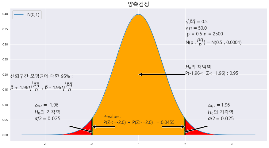
H_0 : p = 0.5(양측 검정)
p-value : 0.0455
alpha : 0.05
p-value < alpha ==> 0.0455 > 0.05 ==> 귀무가설 H_0 : p = 0.5는 기각한다. 즉 , 찬성율이 0.5가 된다는 주장이 틀렸다.
2> 1000명을 상대로 여론조사를 실시하여 520명이 이 정책에 찬성하였다.
x = np.arange(-5,5 , .001)

fig = plt.figure(figsize=(15,8))
ax = sns.lineplot(x , stats.norm.pdf(x, loc=0 , scale =1)) #정의역 범위 , 평균 = 0 , 표준편차 =1 인 정규분포 플롯

# trust = 95 #신뢰도

ax.set_title('양측검정' ,fontsize = 18)
RATIO = round(520/1000 , 4)
n = 1000
MEANS = 0.5
STDS = round(math.sqrt((MEANS * (1-MEANS) / n)),4)


#==========================================귀무가설 기각과 채택 ====================================================
trust = 95 #신뢰도_유의수준

t_1  = round(scipy.stats.norm.ppf(1 - (1-(trust/100))/2) ,3 )


ax.fill_between(x, stats.norm.pdf(x, loc=0 , scale =1) , 0 , where = (x<=t_1) & (x>=-t_1) , facecolor = 'orange') # x값 , y값 , 0 , x<=0 인곳 , 색깔
area = scipy.stats.norm.cdf(t_1) - scipy.stats.norm.cdf(-t_1)

plt.annotate('' , xy=(0, .2), xytext=(2 , .2)  , arrowprops = dict(facecolor = 'black'))
ax.text(2 , .2, r'$H_{0}$의 채택역' +f'\nP({-t_1}<=Z<={t_1}) : {round(area,4)}',fontsize=15)

annotate_len = stats.norm.pdf(t_1, loc=0 , scale =1) /2
ax.vlines(x= t_1, ymin= 0 , ymax= stats.norm.pdf(t_1, loc=0 , scale =1) , color = 'green' , linestyle ='solid' , label ='{}'.format(2))
ax.vlines(x= -t_1, ymin= 0 , ymax= stats.norm.pdf(-t_1, loc=0 , scale =1) , color = 'green' , linestyle ='solid' , label ='{}'.format(2))
area = round((1-area)/2 ,3)
ax.text(1 + t_1 , annotate_len+0.02 , r'$z_{\alpha/2} = $' + f'{t_1}\n' + r'$H_{0}$의 기각역' + f'\n'+ r'$\alpha/2 = {%.3f}$' % area,fontsize=15)
ax.text(-2.5 -t_1 , annotate_len+0.02 , r'$z_{\alpha/2} = $' + f'{-t_1}\n' + r'$H_{0}$의 기각역' + f'\n'+ r'$\alpha/2 = {%.3f}$' % area,fontsize=15)


plt.annotate('' , xy=(t_1, annotate_len-0.02), xytext=(t_1+ 1 , annotate_len)  , arrowprops = dict(facecolor = 'black'))
plt.annotate('' , xy=(-t_1, annotate_len-0.02), xytext=(-1-t_1 , annotate_len)  , arrowprops = dict(facecolor = 'black'))


ax.text(-5.5 , .15, f'신뢰구간 모평균에 대한 {trust}% : \n' + r'$\widehat{p}$' +f' + {t_1}' + r'$\sqrt{\dfrac{\widehat{p}\widehat{q}}{n}}$' +' , '+ r'$\widehat{p}$' +f' - {t_1}' + r'$\sqrt{\dfrac{\widehat{p}\widehat{q}}{n}}$',fontsize=15)


# ax.text(-5.5 , .25,  r'신뢰구간 L = $2*{%.3f}\dfrac{\sigma}{\sqrt{n}} $' % t_1 ,fontsize=15)
#
# ax.text(-5.5 , .3,  r'오차한계 = ${%.3f}\dfrac{\sigma}{\sqrt{n}} $' % t_1,fontsize=15)


#============================================표본평균의 정규분포화 =========================================================

z_1 = round((RATIO-MEANS)/STDS,4)
print(z_1)
z_1 = abs(z_1)
# # z_2 = round((34.5 - 35) / math.sqrt(5.5**2 / 25) , 2)
# z_1 = round(scipy.stats.norm.ppf(1 - (1-(trust/100))/2) ,3 )

ax.fill_between(x, stats.norm.pdf(x, loc=0 , scale =1) , 0 , where = (x<=-z_1) | (x>=z_1) , facecolor = 'skyblue') # x값 , y값 , 0 , x<=0 인곳 , 색깔
ax.fill_between(x, stats.norm.pdf(x, loc=0 , scale =1) , 0 , where = (x>=t_1) | (x<=-t_1) , facecolor = 'red') # x값 , y값 , 0 , x<=0 인곳 , 색깔
area = scipy.stats.norm.cdf(-z_1) + 1 - scipy.stats.norm.cdf(z_1)


ax.vlines(x= z_1, ymin= 0 , ymax= stats.norm.pdf(z_1, loc=0 , scale =1) , color = 'black' , linestyle ='solid' , label ='{}'.format(2))
ax.vlines(x= -z_1, ymin= 0 , ymax= stats.norm.pdf(-z_1, loc=0 , scale =1) , color = 'black' , linestyle ='solid' , label ='{}'.format(2))

annotate_len = stats.norm.pdf(z_1, loc=0 , scale =1) /2
plt.annotate('' , xy=(z_1, annotate_len), xytext=(z_1- 1 , annotate_len)  , arrowprops = dict(facecolor = 'black'))
plt.annotate('' , xy=(-z_1, annotate_len), xytext=(1-z_1 , annotate_len)  , arrowprops = dict(facecolor = 'black'))
ax.text(-1.5 , annotate_len+0.01 , f'P-value : \nP(Z<={-z_1}) + P(Z>={z_1})  = {round(area,4)}',fontsize=15)
# ax.text(0 , annotate_len+0.01 ,f'P(Z>={-z_1})',fontsize=15)


ax.text(2 , .3,  r'$\sqrt{\widehat{p}\widehat{q}} = $' + f'{round(math.sqrt(RATIO * (1-RATIO)),3)}\n'  + r'$\sqrt{n} = $' + f'{round(math.sqrt(n),2)} \n p = {MEANS} n = {n} \n' + r'N(p , ' + r'$\dfrac{pq}{n}) = $' + f'N({MEANS} , {round(MEANS*(1-MEANS)/ n ,8)})',fontsize=15)


b= 'N(0,1)'

plt.legend([b] , fontsize = 15 , loc='upper left')

H_0 : p = 0.5(양측 검정)
p-value : 0.2056
alpha : 0.05
p-value > alpha ==> 0.2056 > 0.05 ==> 귀무가설 H_0 : p = 0.5는 채택한다. 즉 , 찬성율이 0.5가 된다는 주장이 맞았다.
13. 한 포털 사이트는 우리나라 20세 이상의 성인들 중에서 인터넷 신문을 이용하는 사람의 비율이 54.5%를 초과한다고 하였다. 이를 알아보기 위하여 427명을 임의로 선정하여 인터넷 신문의 이용 여부를 조사한 결과 256명이 인터넷 신문을 이용한다고 응답하였다. 이 자료를 근거로 p-value 값을 구하여 인터넷 신문의 이용률이 54.5%를 초과하는지 유의수준 5%에서 조사하라
|X = 256/427
n = 427
trust = 95
H_0 : p <= 0.545(상단측 검정)
x = np.arange(-5,5 , .001)

fig = plt.figure(figsize=(15,8))
ax = sns.lineplot(x , stats.norm.pdf(x, loc=0 , scale =1)) #정의역 범위 , 평균 = 0 , 표준편차 =1 인 정규분포 플롯

# trust = 95 #신뢰도

ax.set_title('상단측검정' ,fontsize = 18)
RATIO = round(256/427 , 4)
n = 427
MEANS = 0.545
STDS = round(math.sqrt((MEANS * (1-MEANS) / n)),4)


#==========================================귀무가설 기각과 채택 ====================================================
trust = 95 #신뢰도_유의수준

t_1  = round(scipy.stats.norm.ppf(1 - (1-(trust/100))/2) ,3 )


ax.fill_between(x, stats.norm.pdf(x, loc=0 , scale =1) , 0 , where = (x<=t_1)  , facecolor = 'orange') # x값 , y값 , 0 , x<=0 인곳 , 색깔
area = scipy.stats.norm.cdf(t_1) - scipy.stats.norm.cdf(-t_1)

plt.annotate('' , xy=(0, .2), xytext=(2 , .2)  , arrowprops = dict(facecolor = 'black'))
ax.text(2 , .2, r'$H_{0}$의 채택역' +f'\nP(Z<={t_1}) : {round(area,4)}',fontsize=15)

annotate_len = stats.norm.pdf(t_1, loc=0 , scale =1) /2
ax.vlines(x= t_1, ymin= 0 , ymax= stats.norm.pdf(t_1, loc=0 , scale =1) , color = 'green' , linestyle ='solid' , label ='{}'.format(2))
# ax.vlines(x= -t_1, ymin= 0 , ymax= stats.norm.pdf(-t_1, loc=0 , scale =1) , color = 'green' , linestyle ='solid' , label ='{}'.format(2))
area = round((1-area),2)
ax.text(1 + t_1 , annotate_len+0.02 , r'$z_{\alpha} = $' + f'{t_1}\n' + r'$H_{0}$의 기각역' + f'\n'+ r'$\alpha = {%.3f}$' % area,fontsize=15)
# ax.text(-2.5 -t_1 , annotate_len+0.02 , r'$z_{\alpha/2} = $' + f'{-t_1}\n' + r'$H_{0}$의 기각역' + f'\n'+ r'$\alpha/2 = {%.3f}$' % area,fontsize=15)


plt.annotate('' , xy=(t_1, annotate_len-0.02), xytext=(t_1+ 1 , annotate_len)  , arrowprops = dict(facecolor = 'black'))
# plt.annotate('' , xy=(-t_1, annotate_len-0.02), xytext=(-1-t_1 , annotate_len)  , arrowprops = dict(facecolor = 'black'))


ax.text(-5.5 , .15, f'신뢰구간 모평균에 대한 {trust}% : \n' + r'$\widehat{p}$' +f' + {t_1}' + r'$\sqrt{\dfrac{\widehat{p}\widehat{q}}{n}}$' +' , '+ r'$\widehat{p}$' +f' - {t_1}' + r'$\sqrt{\dfrac{\widehat{p}\widehat{q}}{n}}$',fontsize=15)


# ax.text(-5.5 , .25,  r'신뢰구간 L = $2*{%.3f}\dfrac{\sigma}{\sqrt{n}} $' % t_1 ,fontsize=15)
#
# ax.text(-5.5 , .3,  r'오차한계 = ${%.3f}\dfrac{\sigma}{\sqrt{n}} $' % t_1,fontsize=15)


#============================================표본평균의 정규분포화 =========================================================

z_1 = round((RATIO-MEANS)/STDS,4)
print(z_1)
z_1 = abs(z_1)
# # z_2 = round((34.5 - 35) / math.sqrt(5.5**2 / 25) , 2)
# z_1 = round(scipy.stats.norm.ppf(1 - (1-(trust/100))/2) ,3 )

ax.fill_between(x, stats.norm.pdf(x, loc=0 , scale =1) , 0 , where =  (x>=z_1) , facecolor = 'skyblue') # x값 , y값 , 0 , x<=0 인곳 , 색깔
ax.fill_between(x, stats.norm.pdf(x, loc=0 , scale =1) , 0 , where = (x>=t_1)  , facecolor = 'red') # x값 , y값 , 0 , x<=0 인곳 , 색깔
area = 1 - scipy.stats.norm.cdf(z_1)


ax.vlines(x= z_1, ymin= 0 , ymax= stats.norm.pdf(z_1, loc=0 , scale =1) , color = 'black' , linestyle ='solid' , label ='{}'.format(2))
# ax.vlines(x= -z_1, ymin= 0 , ymax= stats.norm.pdf(-z_1, loc=0 , scale =1) , color = 'black' , linestyle ='solid' , label ='{}'.format(2))

annotate_len = stats.norm.pdf(z_1, loc=0 , scale =1) /2
plt.annotate('' , xy=(z_1, annotate_len), xytext=(z_1- 1 , annotate_len)  , arrowprops = dict(facecolor = 'black'))
# plt.annotate('' , xy=(-z_1, annotate_len), xytext=(1-z_1 , annotate_len)  , arrowprops = dict(facecolor = 'black'))
ax.text(-1.5 , annotate_len+0.01 , f'P-value : \nP(Z>={z_1})  = {round(area,4)}',fontsize=15)
# ax.text(0 , annotate_len+0.01 ,f'P(Z>={-z_1})',fontsize=15)


ax.text(2 , .3,  r'$\sqrt{\widehat{p}\widehat{q}} = $' + f'{round(math.sqrt(RATIO * (1-RATIO)),3)}\n'  + r'$\sqrt{n} = $' + f'{round(math.sqrt(n),2)} \n p = {MEANS} n = {n} \n' + r'N(p , ' + r'$\dfrac{pq}{n}) = $' + f'N({MEANS} , {round(MEANS*(1-MEANS)/ n ,8)})',fontsize=15)


b= 'N(0,1)'

plt.legend([b] , fontsize = 15 , loc='upper left')

H_0 : p <= 0.545(상단측 검정)
p-value : 0.0119
alpha : 0.05
p-value < alpha ==> 0.0119 < 0.05 ==> 귀무가설 H_0 : p <= 0.545 는 기각한다. 즉 , 인터넷 신문의 이용률이 54.5%를 초과한다.
14. 어느 지역에 거주하는 외국인을 상대로 조사한 보고서에 따르면, 한국인을 친근하게 느낀다고 응답한 비율이 34.4%를 넘지 않는다고 한다. 이것을 알아보기 위하여 그 지역에 거주한느 외국인 450명을 조사한 결과, 139명이 친근하게 느낀다고 응답하였다. 이 자료를 근거로 p-value 값을 구하여 보고서의 내용에 대하여 유의수준 5%에서 조사하라.
|X = 139/450
n = 450
p = 0.344
H_0 : p >= 0.344(하단측 검정)
x = np.arange(-5,5 , .001)

fig = plt.figure(figsize=(15,8))
ax = sns.lineplot(x , stats.norm.pdf(x, loc=0 , scale =1)) #정의역 범위 , 평균 = 0 , 표준편차 =1 인 정규분포 플롯

# trust = 95 #신뢰도

ax.set_title('하단측검정' ,fontsize = 18)
RATIO = round(139/450 , 4)
n = 450
MEANS = 0.344
STDS = round(math.sqrt((MEANS * (1-MEANS) / n)),4)


#==========================================귀무가설 기각과 채택 ====================================================
trust = 95 #신뢰도_유의수준

t_1  = round(scipy.stats.norm.ppf(1 - (1-(trust/100))/2) ,3 )


ax.fill_between(x, stats.norm.pdf(x, loc=0 , scale =1) , 0 , where = (x>=-t_1) , facecolor = 'orange') # x값 , y값 , 0 , x<=0 인곳 , 색깔
area = scipy.stats.norm.cdf(t_1) - scipy.stats.norm.cdf(-t_1)

plt.annotate('' , xy=(0, .2), xytext=(2 , .2)  , arrowprops = dict(facecolor = 'black'))
ax.text(2 , .2, r'$H_{0}$의 채택역' +f'\nP({-t_1}<=Z) : {round(area,4)}',fontsize=15)

annotate_len = stats.norm.pdf(t_1, loc=0 , scale =1) /2
# ax.vlines(x= t_1, ymin= 0 , ymax= stats.norm.pdf(t_1, loc=0 , scale =1) , color = 'green' , linestyle ='solid' , label ='{}'.format(2))
ax.vlines(x= -t_1, ymin= 0 , ymax= stats.norm.pdf(-t_1, loc=0 , scale =1) , color = 'green' , linestyle ='solid' , label ='{}'.format(2))
area = round((1-area) ,3)
# ax.text(1 + t_1 , annotate_len+0.02 , r'$z_{\alpha/2} = $' + f'{t_1}\n' + r'$H_{0}$의 기각역' + f'\n'+ r'$\alpha/2 = {%.3f}$' % area,fontsize=15)
ax.text(-2.5 -t_1 , annotate_len+0.02 , r'$z_{\alpha} = $' + f'{-t_1}\n' + r'$H_{0}$의 기각역' + f'\n'+ r'$\alpha = {%.3f}$' % area,fontsize=15)


# plt.annotate('' , xy=(t_1, annotate_len-0.02), xytext=(t_1+ 1 , annotate_len)  , arrowprops = dict(facecolor = 'black'))
plt.annotate('' , xy=(-t_1, annotate_len-0.02), xytext=(-1-t_1 , annotate_len)  , arrowprops = dict(facecolor = 'black'))


ax.text(-5.5 , .15, f'신뢰구간 모평균에 대한 {trust}% : \n' + r'$\widehat{p}$' +f' + {t_1}' + r'$\sqrt{\dfrac{\widehat{p}\widehat{q}}{n}}$' +' , '+ r'$\widehat{p}$' +f' - {t_1}' + r'$\sqrt{\dfrac{\widehat{p}\widehat{q}}{n}}$',fontsize=15)


# ax.text(-5.5 , .25,  r'신뢰구간 L = $2*{%.3f}\dfrac{\sigma}{\sqrt{n}} $' % t_1 ,fontsize=15)
#
# ax.text(-5.5 , .3,  r'오차한계 = ${%.3f}\dfrac{\sigma}{\sqrt{n}} $' % t_1,fontsize=15)


#============================================표본평균의 정규분포화 =========================================================

z_1 = round((RATIO-MEANS)/STDS,4)
print(z_1)
z_1 = abs(z_1)
# # z_2 = round((34.5 - 35) / math.sqrt(5.5**2 / 25) , 2)
# z_1 = round(scipy.stats.norm.ppf(1 - (1-(trust/100))/2) ,3 )

ax.fill_between(x, stats.norm.pdf(x, loc=0 , scale =1) , 0 , where = (x<=-z_1) , facecolor = 'skyblue') # x값 , y값 , 0 , x<=0 인곳 , 색깔
ax.fill_between(x, stats.norm.pdf(x, loc=0 , scale =1) , 0 , where =  (x<=-t_1) , facecolor = 'red') # x값 , y값 , 0 , x<=0 인곳 , 색깔
area = scipy.stats.norm.cdf(-z_1)


# ax.vlines(x= z_1, ymin= 0 , ymax= stats.norm.pdf(z_1, loc=0 , scale =1) , color = 'black' , linestyle ='solid' , label ='{}'.format(2))
ax.vlines(x= -z_1, ymin= 0 , ymax= stats.norm.pdf(-z_1, loc=0 , scale =1) , color = 'black' , linestyle ='solid' , label ='{}'.format(2))

annotate_len = stats.norm.pdf(z_1, loc=0 , scale =1) /2
# plt.annotate('' , xy=(z_1, annotate_len), xytext=(z_1- 1 , annotate_len)  , arrowprops = dict(facecolor = 'black'))
plt.annotate('' , xy=(-z_1, annotate_len), xytext=(1-z_1 , annotate_len)  , arrowprops = dict(facecolor = 'black'))
ax.text(-1.5 , annotate_len+0.01 , f'P-value : \nP(Z<={-z_1})  = {round(area,4)}',fontsize=15)
# ax.text(0 , annotate_len+0.01 ,f'P(Z>={-z_1})',fontsize=15)


ax.text(2 , .3,  r'$\sqrt{\widehat{p}\widehat{q}} = $' + f'{round(math.sqrt(RATIO * (1-RATIO)),3)}\n'  + r'$\sqrt{n} = $' + f'{round(math.sqrt(n),2)} \n p = {MEANS} n = {n} \n' + r'N(p , ' + r'$\dfrac{pq}{n}) = $' + f'N({MEANS} , {round(MEANS*(1-MEANS)/ n ,8)})',fontsize=15)


b= 'N(0,1)'

plt.legend([b] , fontsize = 15 , loc='upper left')

H_0 : p >= 0.344(상단측 검정)
p-value : 0.0586
alpha : 0.05
p-value > alpha ==> 0.0586 < 0.05 ==> 귀무가설 H_0 : p >= 0.344 는 채택한다. 즉 , 외국인중 한국인을 친근하다고 느끼는 비율은 34.4%를 넘는다.
'기초통계 > 대표본 가설검정' 카테고리의 다른 글
★모평균의 가설 검정★기초통계학-[연습문제 02 -10]
6. 어느 지역에서 일을 하는 건설 노동자의 하루 평균 임금이 14.5만원 인지 알아보기 위하여 이 지역의 건설 노동자 350명을 대상으로 조사한 결과 , 평균 임금이 14.2만원 , 표준편차가 3.5만원 인 것으로 조사되었다. 이 자료를 근거로 평균임금이 14.5 만원 인지 유의수준 10%에서 조사하라.
|X = 14.2
s = 3.5
n = 3.5
trust = 90
H_0 : m = 14.5 (양측검정)
x = np.arange(-5,5 , .001)

fig = plt.figure(figsize=(15,8))
ax = sns.lineplot(x , stats.norm.pdf(x, loc=0 , scale =1)) #정의역 범위 , 평균 = 0 , 표준편차 =1 인 정규분포 플롯

trust = 95 #신뢰도
# MEANS_A = 48.5
# MEANS_B = 50
# MEANS = MEANS_A-MEANS_B
# std_a = 5
# std_b = 5
# n_a = 55
# n_b = 47
# STDS = round(math.sqrt(std_a**2/n_a + std_b**2/n_b),3)
MEANS = 14.2
STDS = 3.5
n = 350

ax.set_title('양측검정' ,fontsize = 18)


#==========================================귀무가설 기각과 채택 ====================================================
trust = 90 #신뢰도_유의수준

t_1  = round(scipy.stats.norm.ppf(1 - (1-(trust/100))/2) ,3 )


ax.fill_between(x, stats.norm.pdf(x, loc=0 , scale =1) , 0 , where = (x<=t_1) & (x>=-t_1) , facecolor = 'orange') # x값 , y값 , 0 , x<=0 인곳 , 색깔
area = scipy.stats.norm.cdf(t_1) - scipy.stats.norm.cdf(-t_1)
ax.fill_between(x, stats.norm.pdf(x, loc=0 , scale =1) , 0 , where = (x>=t_1) | (x<=-t_1) , facecolor = 'red')
plt.annotate('' , xy=(0, .2), xytext=(2 , .2)  , arrowprops = dict(facecolor = 'black'))
ax.text(2 , .2, r'$H_{0}$의 채택역' +f'\nP({-t_1}<=Z<={t_1}) : {round(area,4)}',fontsize=15)

annotate_len = stats.norm.pdf(t_1, loc=0 , scale =1) /2
ax.vlines(x= t_1, ymin= 0 , ymax= stats.norm.pdf(t_1, loc=0 , scale =1) , color = 'green' , linestyle ='solid' , label ='{}'.format(2))
ax.vlines(x= -t_1, ymin= 0 , ymax= stats.norm.pdf(-t_1, loc=0 , scale =1) , color = 'green' , linestyle ='solid' , label ='{}'.format(2))

area = round((1-area)/2 ,3)
ax.text(1 + t_1 , annotate_len+0.02 , r'$z_{\alpha/2} = $' + f'{t_1}\n' + r'$H_{0}$의 기각역' + f'\n'+ r'$\alpha/2 = {%.3f}$' % area,fontsize=15)
ax.text(-2.5 -t_1 , annotate_len+0.02 , r'$z_{\alpha/2} = $' + f'{-t_1}\n' + r'$H_{0}$의 기각역' + f'\n'+ r'$\alpha/2 = {%.3f}$' % area,fontsize=15)


plt.annotate('' , xy=(t_1, annotate_len), xytext=(t_1+ 1 , annotate_len+0.02)  , arrowprops = dict(facecolor = 'black'))
plt.annotate('' , xy=(-t_1, annotate_len), xytext=(-1-t_1 , annotate_len+0.02)  , arrowprops = dict(facecolor = 'black'))


# ax.text(-5.5 , .25, f'신뢰구간 모평균에 대한 {trust}% : \n' + r'$\left( \overline{x}-\overline{y}\right)$' +f'-{t_1}' + r'$\sqrt{\dfrac{\sigma_{1}^{2}}{n}+\dfrac{\sigma_{2} ^{2}}{m}}$' +' , '+ r'$\left( \overline{x}-\overline{y}\right)$' +f'+ {t_1}' + r'$\sqrt{\dfrac{\sigma_{1}^{2}}{n}+\dfrac{\sigma_{2} ^{2}}{m}}$',fontsize=15)

ax.text(-5.5 , .15, f'신뢰구간 모평균에 대한 {trust}% : \n' + r'$\overline{X}$' +f'-{t_1}' + r'$\dfrac{\sigma}{\sqrt{n}},\overline{X}$' + f'+{t_1}' + r'$\dfrac{\sigma}{\sqrt{n}}$ ' ,fontsize=15)
ax.text(-5.5 , .25,  r'신뢰구간 L = $2*{%.3f}\dfrac{\sigma}{\sqrt{n}} $' % t_1 ,fontsize=15)

ax.text(-5.5 , .3,  r'오차한계 = ${%.3f}\dfrac{\sigma}{\sqrt{n}} $' % t_1,fontsize=15)

ax.text(2 , .35,  r'$\overline{X}$ = ' + f'{MEANS}\n' + r'$\sigma = $' + f'{STDS}\n' + r'$\sqrt{n} = $' + f'{round(math.sqrt(n),3)}',fontsize=15)
# ax.text(2 , .35,  r'$\overline{X}_{1}$ = ' +f'{MEANS_A}'+   r' , $\overline{X}_{2}$ = ' +f'{MEANS_B}\n' + r'$\sigma_{1} = $' + f'{std_a}' + r', $\sigma_{2} = $' + f'{std_b}\n' + r'$\sqrt{n} = $' + f'{round(math.sqrt(n_a),3)}' + r', $\sqrt{m} = $' + f'{round(math.sqrt(n_b),3)}',fontsize=15)


#============================================표본평균의 정규분포화 =========================================================
z_1 = round((MEANS-14.5)/ math.sqrt(STDS**2/n) ,2)
# # z_2 = round((34.5 - 35) / math.sqrt(5.5**2 / 25) , 2)
# z_1 = round(scipy.stats.norm.ppf(1 - (1-(trust/100))/2) ,3 )
print(z_1)

z_1 = abs(z_1)
ax.fill_between(x, stats.norm.pdf(x, loc=0 , scale =1) , 0 , where = (x>=z_1) | (x<=-z_1) , facecolor = 'skyblue') # x값 , y값 , 0 , x<=0 인곳 , 색깔
ax.fill_between(x, stats.norm.pdf(x, loc=0 , scale =1) , 0 , where = (x>=t_1) | (x<=-t_1) , facecolor = 'red') # x값 , y값 , 0 , x<=0 인곳 , 색깔
area = scipy.stats.norm.cdf(-z_1) + 1- scipy.stats.norm.cdf(z_1)


ax.vlines(x= -z_1, ymin= 0 , ymax= stats.norm.pdf(-z_1, loc=0 , scale =1) , color = 'black' , linestyle ='solid' , label ='{}'.format(2))
ax.vlines(x= z_1, ymin= 0 , ymax= stats.norm.pdf(z_1, loc=0 , scale =1) , color = 'black' , linestyle ='solid' , label ='{}'.format(2))

annotate_len = stats.norm.pdf(z_1, loc=0 , scale =1) /2
plt.annotate('' , xy=(z_1, annotate_len), xytext=(z_1- 1 , annotate_len)  , arrowprops = dict(facecolor = 'black'))
plt.annotate('' , xy=(-z_1, annotate_len), xytext=(1-z_1 , annotate_len)  , arrowprops = dict(facecolor = 'black'))
ax.text(-1.5 , annotate_len+0.01 , f'P-VALUE: \n  P(Z<={-z_1}) + P(Z>={z_1})  = {round(area,4)}',fontsize=15)


b= 'N(0,1)'

plt.legend([b] , fontsize = 15 , loc='upper left')

p-value : 0.1096
alpha : 0.1
p-value > alpha ==> 0.1096 > 0.1==> 귀무가설 H_0 : m =14.5 는 채택한다.
7. 고무 장난감을 생산하는 한 회사가 지름 60mm인 유아용 고무 원판을 주문받아 제작하였다. 그러나 물건을 받은 주문자는 이 업체에서 생산한 고무 원판의 지름이 60mm에 미치지 않는다고 항의하였다. 이것을 알아보기 위하여, 50개의 고무 원판을 표본조사했더니 다음과 같았다. 이 자료를 근거로 주문자의 주장이 맞는 지 유의수준 5%에서 조사하라.
|X = > NUMPY 활용
s => NUMPY (표본평균의 표준편차)
n = 50
trust = 95
H_0 : m >= 60 (하단측 검정)
H_1 : m < 60
x = np.arange(-5,5 , .001)

fig = plt.figure(figsize=(15,8))
ax = sns.lineplot(x , stats.norm.pdf(x, loc=0 , scale =1)) #정의역 범위 , 평균 = 0 , 표준편차 =1 인 정규분포 플롯

trust = 95 #신뢰도
A = "56.7 64.0 58.2 60.4 63.7 58.0 55.1 54.3 57.8 63.1 61.6 63.2 54.3 54.2 56.2 63.4 57.7 54.2 55.4 60.3 60.2 54.1 60.1 57.1 57.2 61.9 63.2 59.6 60.1 62.1 61.2 56.0 55.9 54.8 58.1 61.5 61.7 61.2 55.8 59.0 62.9 63.9 59.3 60.9 59.0 58.7 61.4 61.8 54.9 57.7"
A = list(map(float, A.split(' ')))
MEANS = np.mean(A)
STDS = np.std(A , ddof=1)
n = len(A)

ax.set_title('하단측검정' ,fontsize = 18)


#==========================================귀무가설 기각과 채택 ====================================================
trust = 95 #신뢰도_유의수준

t_1  = round(scipy.stats.norm.ppf(1 - (1-(trust/100))) ,3 )


ax.fill_between(x, stats.norm.pdf(x, loc=0 , scale =1) , 0 , where = (x>=-t_1)  , facecolor = 'orange') # x값 , y값 , 0 , x<=0 인곳 , 색깔
area = 1- scipy.stats.norm.cdf(-t_1)

plt.annotate('' , xy=(0, .2), xytext=(2 , .2)  , arrowprops = dict(facecolor = 'black'))
ax.text(2 , .2, r'$H_{0}$의 채택역' +f'\nP(Z>={-t_1}) : {round(area,4)}',fontsize=15)

annotate_len = stats.norm.pdf(t_1, loc=0 , scale =1) /2
ax.vlines(x= -t_1, ymin= 0 , ymax= stats.norm.pdf(-t_1, loc=0 , scale =1) , color = 'green' , linestyle ='solid' , label ='{}'.format(2))
# ax.vlines(x= -t_1, ymin= 0 , ymax= stats.norm.pdf(-t_1, loc=0 , scale =1) , color = 'green' , linestyle ='solid' , label ='{}'.format(2))

area = round((1-area) ,3)
# ax.text(1 + t_1 , annotate_len+0.02 , r'$z_{\alpha} = $' + f'{t_1}\n' + r'$H_{0}$의 기각역' + f'\n'+ r'$\alpha = {%.3f}$' % area,fontsize=15)
ax.text(-2.5 -t_1 , annotate_len+0.02 , r'$z_{\alpha/2} = $' + f'{-t_1}\n' + r'$H_{0}$의 기각역' + f'\n'+ r'$\alpha/2 = {%.3f}$' % area,fontsize=15)


# plt.annotate('' , xy=(t_1, annotate_len), xytext=(t_1+ 1 , annotate_len+0.02)  , arrowprops = dict(facecolor = 'black'))
plt.annotate('' , xy=(-t_1, annotate_len), xytext=(-1-t_1 , annotate_len+0.02)  , arrowprops = dict(facecolor = 'black'))


# ax.text(-5.5 , .25, f'신뢰구간 모평균에 대한 {trust}% : \n' + r'$\left( \overline{x}-\overline{y}\right)$' +f'-{t_1}' + r'$\sqrt{\dfrac{\sigma_{1}^{2}}{n}+\dfrac{\sigma_{2} ^{2}}{m}}$' +' , '+ r'$\left( \overline{x}-\overline{y}\right)$' +f'+ {t_1}' + r'$\sqrt{\dfrac{\sigma_{1}^{2}}{n}+\dfrac{\sigma_{2} ^{2}}{m}}$',fontsize=15)

ax.text(-5.5 , .15, f'신뢰구간 모평균에 대한 {trust}% : \n' + r'$\overline{X}$' +f'-{t_1}' + r'$\dfrac{\sigma}{\sqrt{n}},\overline{X}$' + f'+{t_1}' + r'$\dfrac{\sigma}{\sqrt{n}}$ ' ,fontsize=15)
ax.text(-5.5 , .25,  r'신뢰구간 L = $2*{%.3f}\dfrac{\sigma}{\sqrt{n}} $' % t_1 ,fontsize=15)

ax.text(-5.5 , .3,  r'오차한계 = ${%.3f}\dfrac{\sigma}{\sqrt{n}} $' % t_1,fontsize=15)

ax.text(2 , .35,  r'$\overline{X}$ = ' + f'{MEANS}\n' + r'$\sigma = $' + f'{STDS}\n' + r'$\sqrt{n} = $' + f'{round(math.sqrt(n),3)}',fontsize=15)
# ax.text(2 , .35,  r'$\overline{X}_{1}$ = ' +f'{MEANS_A}'+   r' , $\overline{X}_{2}$ = ' +f'{MEANS_B}\n' + r'$\sigma_{1} = $' + f'{std_a}' + r', $\sigma_{2} = $' + f'{std_b}\n' + r'$\sqrt{n} = $' + f'{round(math.sqrt(n_a),3)}' + r', $\sqrt{m} = $' + f'{round(math.sqrt(n_b),3)}',fontsize=15)


#============================================표본평균의 정규분포화 =========================================================
z_1 = round((MEANS-60)/ math.sqrt(STDS**2/n) ,2)
# # z_2 = round((34.5 - 35) / math.sqrt(5.5**2 / 25) , 2)
# z_1 = round(scipy.stats.norm.ppf(1 - (1-(trust/100))/2) ,3 )
print(z_1)
#
# z_1 = abs(z_1)
ax.fill_between(x, stats.norm.pdf(x, loc=0 , scale =1) , 0 , where = (x<=z_1) , facecolor = 'skyblue') # x값 , y값 , 0 , x<=0 인곳 , 색깔
ax.fill_between(x, stats.norm.pdf(x, loc=0 , scale =1) , 0 , where = (x<=-t_1) , facecolor = 'red') # x값 , y값 , 0 , x<=0 인곳 , 색깔
area =  scipy.stats.norm.cdf(z_1)


# ax.vlines(x= -z_1, ymin= 0 , ymax= stats.norm.pdf(-z_1, loc=0 , scale =1) , color = 'black' , linestyle ='solid' , label ='{}'.format(2))
ax.vlines(x= z_1, ymin= 0 , ymax= stats.norm.pdf(z_1, loc=0 , scale =1) , color = 'black' , linestyle ='solid' , label ='{}'.format(2))

annotate_len = stats.norm.pdf(z_1, loc=0 , scale =1) /2
plt.annotate('' , xy=(z_1, annotate_len), xytext=( -3 - z_1 , annotate_len)  , arrowprops = dict(facecolor = 'black'))
# plt.annotate('' , xy=(-z_1, annotate_len), xytext=(1-z_1 , annotate_len)  , arrowprops = dict(facecolor = 'black'))
ax.text(-1.5 , annotate_len+0.01 , f'P-VALUE: \n  P( P(Z<={z_1})  = {round(area,4)}',fontsize=15)


b= 'N(0,1)'

plt.legend([b] , fontsize = 15 , loc='upper left')

p-value : 0.0154
alpha : 0.05
p-value < alpha ==> 0.0154 < 0.5 ==> 귀무가설 H_0 : m >= 60 (하단측 검정) 는 기각한다. 따라서 60mm에 미치지 않는다는 가설은 채택한다.(주문자의 말이 맞다.)
8. 우리나라 사람의 커피 소비량은 1인당 연평균 484잔을 초과한다고 한다. 이를 알아보기 위하여 200명을 임의로 선정하여 커피 소비량을 조사한 결과, 1인당 소비하는 커피는 연평균 486잔 그리고 표준편차는 16.54잔 이었다. 이 자료를 근거로 p-value 값 구하여 커피 소비량이 1인당 484잔을 초과하는지 유의수준 5%에서 조사하라.
|X = 486
s = 16.54
n = 200
trust = 95
H_0 : M <= 484 (상단측 검정)
x = np.arange(-5,5 , .001)

fig = plt.figure(figsize=(15,8))
ax = sns.lineplot(x , stats.norm.pdf(x, loc=0 , scale =1)) #정의역 범위 , 평균 = 0 , 표준편차 =1 인 정규분포 플롯

trust = 95 #신뢰도
# MEANS_A = 48.5
# MEANS_B = 50
# MEANS = MEANS_A-MEANS_B
# std_a = 5
# std_b = 5
# n_a = 55
# n_b = 47
# STDS = round(math.sqrt(std_a**2/n_a + std_b**2/n_b),3)
MEANS = 486
STDS = 16.54
n = 200

ax.set_title('상단측검정' ,fontsize = 18)


#==========================================귀무가설 기각과 채택 ====================================================
trust = 95 #신뢰도_유의수준

t_1  = round(scipy.stats.norm.ppf(1 - (1-(trust/100))) ,3 )


ax.fill_between(x, stats.norm.pdf(x, loc=0 , scale =1) , 0 , where = (x<=t_1)  , facecolor = 'orange') # x값 , y값 , 0 , x<=0 인곳 , 색깔
area = scipy.stats.norm.cdf(t_1)

plt.annotate('' , xy=(0, .2), xytext=(2 , .2)  , arrowprops = dict(facecolor = 'black'))
ax.text(2 , .2, r'$H_{0}$의 채택역' +f'\nP(Z<={t_1}) : {round(area,4)}',fontsize=15)

annotate_len = stats.norm.pdf(t_1, loc=0 , scale =1) /2
ax.vlines(x= t_1, ymin= 0 , ymax= stats.norm.pdf(t_1, loc=0 , scale =1) , color = 'green' , linestyle ='solid' , label ='{}'.format(2))
# ax.vlines(x= -t_1, ymin= 0 , ymax= stats.norm.pdf(-t_1, loc=0 , scale =1) , color = 'green' , linestyle ='solid' , label ='{}'.format(2))

area = round((1-area) ,3)
ax.text(1 + t_1 , annotate_len+0.02 , r'$z_{\alpha} = $' + f'{t_1}\n' + r'$H_{0}$의 기각역' + f'\n'+ r'$\alpha = {%.3f}$' % area,fontsize=15)
# ax.text(-2.5 -t_1 , annotate_len+0.02 , r'$z_{\alpha/2} = $' + f'{-t_1}\n' + r'$H_{0}$의 기각역' + f'\n'+ r'$\alpha/2 = {%.3f}$' % area,fontsize=15)


plt.annotate('' , xy=(t_1, annotate_len), xytext=(t_1+ 1 , annotate_len+0.02)  , arrowprops = dict(facecolor = 'black'))
# plt.annotate('' , xy=(-t_1, annotate_len), xytext=(-1-t_1 , annotate_len+0.02)  , arrowprops = dict(facecolor = 'black'))


# ax.text(-5.5 , .25, f'신뢰구간 모평균에 대한 {trust}% : \n' + r'$\left( \overline{x}-\overline{y}\right)$' +f'-{t_1}' + r'$\sqrt{\dfrac{\sigma_{1}^{2}}{n}+\dfrac{\sigma_{2} ^{2}}{m}}$' +' , '+ r'$\left( \overline{x}-\overline{y}\right)$' +f'+ {t_1}' + r'$\sqrt{\dfrac{\sigma_{1}^{2}}{n}+\dfrac{\sigma_{2} ^{2}}{m}}$',fontsize=15)

ax.text(-5.5 , .15, f'신뢰구간 모평균에 대한 {trust}% : \n' + r'$\overline{X}$' +f'-{t_1}' + r'$\dfrac{\sigma}{\sqrt{n}},\overline{X}$' + f'+{t_1}' + r'$\dfrac{\sigma}{\sqrt{n}}$ ' ,fontsize=15)
ax.text(-5.5 , .25,  r'신뢰구간 L = $2*{%.3f}\dfrac{\sigma}{\sqrt{n}} $' % t_1 ,fontsize=15)

ax.text(-5.5 , .3,  r'오차한계 = ${%.3f}\dfrac{\sigma}{\sqrt{n}} $' % t_1,fontsize=15)

ax.text(2 , .35,  r'$\overline{X}$ = ' + f'{MEANS}\n' + r'$\sigma = $' + f'{STDS}\n' + r'$\sqrt{n} = $' + f'{round(math.sqrt(n),3)}',fontsize=15)
# ax.text(2 , .35,  r'$\overline{X}_{1}$ = ' +f'{MEANS_A}'+   r' , $\overline{X}_{2}$ = ' +f'{MEANS_B}\n' + r'$\sigma_{1} = $' + f'{std_a}' + r', $\sigma_{2} = $' + f'{std_b}\n' + r'$\sqrt{n} = $' + f'{round(math.sqrt(n_a),3)}' + r', $\sqrt{m} = $' + f'{round(math.sqrt(n_b),3)}',fontsize=15)


#============================================표본평균의 정규분포화 =========================================================
z_1 = round((MEANS-484)/ math.sqrt(STDS**2/n) ,2)
# # z_2 = round((34.5 - 35) / math.sqrt(5.5**2 / 25) , 2)
# z_1 = round(scipy.stats.norm.ppf(1 - (1-(trust/100))/2) ,3 )
print(z_1)

z_1 = abs(z_1)
ax.fill_between(x, stats.norm.pdf(x, loc=0 , scale =1) , 0 , where = (x>=z_1) , facecolor = 'skyblue') # x값 , y값 , 0 , x<=0 인곳 , 색깔
ax.fill_between(x, stats.norm.pdf(x, loc=0 , scale =1) , 0 , where = (x>=t_1) , facecolor = 'red') # x값 , y값 , 0 , x<=0 인곳 , 색깔
area =  1- scipy.stats.norm.cdf(z_1)


# ax.vlines(x= -z_1, ymin= 0 , ymax= stats.norm.pdf(-z_1, loc=0 , scale =1) , color = 'black' , linestyle ='solid' , label ='{}'.format(2))
ax.vlines(x= z_1, ymin= 0 , ymax= stats.norm.pdf(z_1, loc=0 , scale =1) , color = 'black' , linestyle ='solid' , label ='{}'.format(2))

annotate_len = stats.norm.pdf(z_1, loc=0 , scale =1) /2
plt.annotate('' , xy=(z_1, annotate_len), xytext=(z_1- 1 , annotate_len)  , arrowprops = dict(facecolor = 'black'))
# plt.annotate('' , xy=(-z_1, annotate_len), xytext=(1-z_1 , annotate_len)  , arrowprops = dict(facecolor = 'black'))
ax.text(-1.5 , annotate_len+0.01 , f'P-VALUE: \n  P(Z>={z_1})  = {round(area,4)}',fontsize=15)


b= 'N(0,1)'

plt.legend([b] , fontsize = 15 , loc='upper left')

p-value : 0.0436
alpha : 0.05
p-value < alpha ==> 0.0436 < 0.05 ==> 귀무가설 H_0 : m <= 484 (상단측 검정) 는 기각한다. 따라서 1인당 484잔을 초과한다는 가설을 채택한다.
9. 한 청소년 실태 조사 보고서에 따르면 , 중소도시에 거주하는 청소년이 휴일에 봉사활동이나 동아리 활동을 하는 평균 시간은 76분이라고 한다. 이를 알아보기 위하여 전국의 중소도시에 거주하는 청소년 400명의 봉사활동 또는 동아리 활동 시간을 조사한 결과, 평균 75.4시간, 표준편차 5.8시간이었다. 이 자료를 근거로 봉사활동 또는 동아리 활동 시간이 평균 76분인지 유의수준 5%에서 조사하라.
|X = 75.4
s = 5.8
n = 400
trust = 95
H_0 : m == 76 (양측검정)
x = np.arange(-5,5 , .001)

fig = plt.figure(figsize=(15,8))
ax = sns.lineplot(x , stats.norm.pdf(x, loc=0 , scale =1)) #정의역 범위 , 평균 = 0 , 표준편차 =1 인 정규분포 플롯

trust = 95 #신뢰도
# MEANS_A = 48.5
# MEANS_B = 50
# MEANS = MEANS_A-MEANS_B
# std_a = 5
# std_b = 5
# n_a = 55
# n_b = 47
# STDS = round(math.sqrt(std_a**2/n_a + std_b**2/n_b),3)
MEANS = 75.4
STDS = 5.8
n = 400

ax.set_title('양측검정' ,fontsize = 18)


#==========================================귀무가설 기각과 채택 ====================================================
trust = 95 #신뢰도_유의수준

t_1  = round(scipy.stats.norm.ppf(1 - (1-(trust/100))/2) ,3 )


ax.fill_between(x, stats.norm.pdf(x, loc=0 , scale =1) , 0 , where = (x<=t_1) & (x>=-t_1) , facecolor = 'orange') # x값 , y값 , 0 , x<=0 인곳 , 색깔
area = scipy.stats.norm.cdf(t_1) - scipy.stats.norm.cdf(-t_1)
ax.fill_between(x, stats.norm.pdf(x, loc=0 , scale =1) , 0 , where = (x>=t_1) | (x<=-t_1) , facecolor = 'red')
plt.annotate('' , xy=(0, .2), xytext=(2 , .2)  , arrowprops = dict(facecolor = 'black'))
ax.text(2 , .2, r'$H_{0}$의 채택역' +f'\nP({-t_1}<=Z<={t_1}) : {round(area,4)}',fontsize=15)

annotate_len = stats.norm.pdf(t_1, loc=0 , scale =1) /2
ax.vlines(x= t_1, ymin= 0 , ymax= stats.norm.pdf(t_1, loc=0 , scale =1) , color = 'green' , linestyle ='solid' , label ='{}'.format(2))
ax.vlines(x= -t_1, ymin= 0 , ymax= stats.norm.pdf(-t_1, loc=0 , scale =1) , color = 'green' , linestyle ='solid' , label ='{}'.format(2))

area = round((1-area)/2 ,3)
ax.text(1 + t_1 , annotate_len+0.02 , r'$z_{\alpha/2} = $' + f'{t_1}\n' + r'$H_{0}$의 기각역' + f'\n'+ r'$\alpha/2 = {%.3f}$' % area,fontsize=15)
ax.text(-2.5 -t_1 , annotate_len+0.02 , r'$z_{\alpha/2} = $' + f'{-t_1}\n' + r'$H_{0}$의 기각역' + f'\n'+ r'$\alpha/2 = {%.3f}$' % area,fontsize=15)


plt.annotate('' , xy=(t_1, annotate_len), xytext=(t_1+ 1 , annotate_len+0.02)  , arrowprops = dict(facecolor = 'black'))
plt.annotate('' , xy=(-t_1, annotate_len), xytext=(-1-t_1 , annotate_len+0.02)  , arrowprops = dict(facecolor = 'black'))


# ax.text(-5.5 , .25, f'신뢰구간 모평균에 대한 {trust}% : \n' + r'$\left( \overline{x}-\overline{y}\right)$' +f'-{t_1}' + r'$\sqrt{\dfrac{\sigma_{1}^{2}}{n}+\dfrac{\sigma_{2} ^{2}}{m}}$' +' , '+ r'$\left( \overline{x}-\overline{y}\right)$' +f'+ {t_1}' + r'$\sqrt{\dfrac{\sigma_{1}^{2}}{n}+\dfrac{\sigma_{2} ^{2}}{m}}$',fontsize=15)

ax.text(-5.5 , .15, f'신뢰구간 모평균에 대한 {trust}% : \n' + r'$\overline{X}$' +f'-{t_1}' + r'$\dfrac{\sigma}{\sqrt{n}},\overline{X}$' + f'+{t_1}' + r'$\dfrac{\sigma}{\sqrt{n}}$ ' ,fontsize=15)
ax.text(-5.5 , .25,  r'신뢰구간 L = $2*{%.3f}\dfrac{\sigma}{\sqrt{n}} $' % t_1 ,fontsize=15)

ax.text(-5.5 , .3,  r'오차한계 = ${%.3f}\dfrac{\sigma}{\sqrt{n}} $' % t_1,fontsize=15)

ax.text(2 , .35,  r'$\overline{X}$ = ' + f'{MEANS}\n' + r'$\sigma = $' + f'{STDS}\n' + r'$\sqrt{n} = $' + f'{round(math.sqrt(n),3)}',fontsize=15)
# ax.text(2 , .35,  r'$\overline{X}_{1}$ = ' +f'{MEANS_A}'+   r' , $\overline{X}_{2}$ = ' +f'{MEANS_B}\n' + r'$\sigma_{1} = $' + f'{std_a}' + r', $\sigma_{2} = $' + f'{std_b}\n' + r'$\sqrt{n} = $' + f'{round(math.sqrt(n_a),3)}' + r', $\sqrt{m} = $' + f'{round(math.sqrt(n_b),3)}',fontsize=15)


#============================================표본평균의 정규분포화 =========================================================
z_1 = round((MEANS-76)/ math.sqrt(STDS**2/n) ,2)
# # z_2 = round((34.5 - 35) / math.sqrt(5.5**2 / 25) , 2)
# z_1 = round(scipy.stats.norm.ppf(1 - (1-(trust/100))/2) ,3 )
print(z_1)

z_1 = abs(z_1)
ax.fill_between(x, stats.norm.pdf(x, loc=0 , scale =1) , 0 , where = (x>=z_1) | (x<=-z_1) , facecolor = 'skyblue') # x값 , y값 , 0 , x<=0 인곳 , 색깔
ax.fill_between(x, stats.norm.pdf(x, loc=0 , scale =1) , 0 , where = (x>=t_1) | (x<=-t_1) , facecolor = 'red') # x값 , y값 , 0 , x<=0 인곳 , 색깔
area = scipy.stats.norm.cdf(-z_1) + 1- scipy.stats.norm.cdf(z_1)


ax.vlines(x= -z_1, ymin= 0 , ymax= stats.norm.pdf(-z_1, loc=0 , scale =1) , color = 'black' , linestyle ='solid' , label ='{}'.format(2))
ax.vlines(x= z_1, ymin= 0 , ymax= stats.norm.pdf(z_1, loc=0 , scale =1) , color = 'black' , linestyle ='solid' , label ='{}'.format(2))

annotate_len = stats.norm.pdf(z_1, loc=0 , scale =1) /2
plt.annotate('' , xy=(z_1, annotate_len), xytext=(z_1- 1 , annotate_len)  , arrowprops = dict(facecolor = 'black'))
plt.annotate('' , xy=(-z_1, annotate_len), xytext=(1-z_1 , annotate_len)  , arrowprops = dict(facecolor = 'black'))
ax.text(-1.5 , annotate_len+0.01 , f'P-VALUE: \n  P(Z<={-z_1}) + P(Z>={z_1})  = {round(area,4)}',fontsize=15)


b= 'N(0,1)'

plt.legend([b] , fontsize = 15 , loc='upper left')
p-value : 0.0385
alpha : 0.05
p-value < alpha ==> 0.0385 < 0.05 ==> 귀무가설 H_0 : m = 76 (양측 검정) 는 기각한다. 따라서 동아리 활동 시간이 평균 76분이 아니다.