★표본비율의 정규분포화★모비율의 가설 검정★기초통계학-[연습문제 03 -11]
10. 우리나라 아동 대상으로 흡연 경험에 대해 조사결과 경험 있다 비율이 8.9%였다. 이를 알아보기 위하여 3000명 대상으로 조사한 결과 294명이 흡연 경험이 있다고 응답하였다. 이 자료를 근거로 흡연 경험이 있는 아동의 비율이 8.9%인지 유의수준 5%에서 조사하라.
https://knowallworld.tistory.com/306
이항분포에 따른 정규분포의 표준정규분포화★표본비율의 표본분포★기초통계학-[모집단 분포
1.표본비율의 표본분포 EX) 이항 확률변수의 실질적인 응용 ==> 여론조사 생각 ==> 모집단을 구성하는 사람들의 어느 특정 사건을 선호하는 비율(p)를 알기 위하여 n명으로 구성된 표본을 임의 선정
knowallworld.tistory.com

Z = ^p - p / 루트( p*q / n)
^p = 294/3000
p = 0.089
n = 3000
trust = 95
H_0 : p = 0.089(양측 검정)
x = np.arange(-5,5 , .001)

fig = plt.figure(figsize=(15,8))
ax = sns.lineplot(x , stats.norm.pdf(x, loc=0 , scale =1)) #정의역 범위 , 평균 = 0 , 표준편차 =1 인 정규분포 플롯

# trust = 95 #신뢰도

ax.set_title('양측검정' ,fontsize = 18)
RATIO = round(294/3000 , 4)
n = 3000
MEANS = 0.089
STDS = round(math.sqrt((MEANS * (1-MEANS) / n)),4)


#==========================================귀무가설 기각과 채택 ====================================================
trust = 95 #신뢰도_유의수준

t_1  = round(scipy.stats.norm.ppf(1 - (1-(trust/100))/2) ,3 )


ax.fill_between(x, stats.norm.pdf(x, loc=0 , scale =1) , 0 , where = (x<=t_1) & (x>=-t_1) , facecolor = 'orange') # x값 , y값 , 0 , x<=0 인곳 , 색깔
area = scipy.stats.norm.cdf(t_1) - scipy.stats.norm.cdf(-t_1)

plt.annotate('' , xy=(0, .2), xytext=(2 , .2)  , arrowprops = dict(facecolor = 'black'))
ax.text(2 , .2, r'$H_{0}$의 채택역' +f'\nP({-t_1}<=Z<={t_1}) : {round(area,4)}',fontsize=15)

annotate_len = stats.norm.pdf(t_1, loc=0 , scale =1) /2
ax.vlines(x= t_1, ymin= 0 , ymax= stats.norm.pdf(t_1, loc=0 , scale =1) , color = 'green' , linestyle ='solid' , label ='{}'.format(2))
ax.vlines(x= -t_1, ymin= 0 , ymax= stats.norm.pdf(-t_1, loc=0 , scale =1) , color = 'green' , linestyle ='solid' , label ='{}'.format(2))
area = round((1-area)/2 ,3)
ax.text(1 + t_1 , annotate_len+0.02 , r'$z_{\alpha/2} = $' + f'{t_1}\n' + r'$H_{0}$의 기각역' + f'\n'+ r'$\alpha/2 = {%.3f}$' % area,fontsize=15)
ax.text(-2.5 -t_1 , annotate_len+0.02 , r'$z_{\alpha/2} = $' + f'{-t_1}\n' + r'$H_{0}$의 기각역' + f'\n'+ r'$\alpha/2 = {%.3f}$' % area,fontsize=15)


plt.annotate('' , xy=(t_1, annotate_len-0.02), xytext=(t_1+ 1 , annotate_len)  , arrowprops = dict(facecolor = 'black'))
plt.annotate('' , xy=(-t_1, annotate_len-0.02), xytext=(-1-t_1 , annotate_len)  , arrowprops = dict(facecolor = 'black'))


ax.text(-5.5 , .15, f'신뢰구간 모평균에 대한 {trust}% : \n' + r'$\widehat{p}$' +f' + {t_1}' + r'$\sqrt{\dfrac{\widehat{p}\widehat{q}}{n}}$' +' , '+ r'$\widehat{p}$' +f' - {t_1}' + r'$\sqrt{\dfrac{\widehat{p}\widehat{q}}{n}}$',fontsize=15)


# ax.text(-5.5 , .25,  r'신뢰구간 L = $2*{%.3f}\dfrac{\sigma}{\sqrt{n}} $' % t_1 ,fontsize=15)
#
# ax.text(-5.5 , .3,  r'오차한계 = ${%.3f}\dfrac{\sigma}{\sqrt{n}} $' % t_1,fontsize=15)


#============================================표본평균의 정규분포화 =========================================================

z_1 = round((RATIO-MEANS)/STDS,4)
print(z_1)
z_1 = abs(z_1)
# # z_2 = round((34.5 - 35) / math.sqrt(5.5**2 / 25) , 2)
# z_1 = round(scipy.stats.norm.ppf(1 - (1-(trust/100))/2) ,3 )

ax.fill_between(x, stats.norm.pdf(x, loc=0 , scale =1) , 0 , where = (x<=-z_1) | (x>=z_1) , facecolor = 'skyblue') # x값 , y값 , 0 , x<=0 인곳 , 색깔
ax.fill_between(x, stats.norm.pdf(x, loc=0 , scale =1) , 0 , where = (x>=t_1) | (x<=-t_1) , facecolor = 'red') # x값 , y값 , 0 , x<=0 인곳 , 색깔
area = scipy.stats.norm.cdf(-z_1) + 1 - scipy.stats.norm.cdf(z_1)


ax.vlines(x= z_1, ymin= 0 , ymax= stats.norm.pdf(z_1, loc=0 , scale =1) , color = 'black' , linestyle ='solid' , label ='{}'.format(2))
ax.vlines(x= -z_1, ymin= 0 , ymax= stats.norm.pdf(-z_1, loc=0 , scale =1) , color = 'black' , linestyle ='solid' , label ='{}'.format(2))

annotate_len = stats.norm.pdf(z_1, loc=0 , scale =1) /2
plt.annotate('' , xy=(z_1, annotate_len), xytext=(z_1- 1 , annotate_len)  , arrowprops = dict(facecolor = 'black'))
plt.annotate('' , xy=(-z_1, annotate_len), xytext=(1-z_1 , annotate_len)  , arrowprops = dict(facecolor = 'black'))
ax.text(-1.5 , annotate_len+0.01 , f'P-value : \nP(Z<={-z_1}) + P(Z>={z_1})  = {round(area,4)}',fontsize=15)
# ax.text(0 , annotate_len+0.01 ,f'P(Z>={-z_1})',fontsize=15)


ax.text(2 , .3,  r'$\sqrt{\widehat{p}\widehat{q}} = $' + f'{round(math.sqrt(RATIO * (1-RATIO)),3)}\n'  + r'$\sqrt{n} = $' + f'{round(math.sqrt(n),2)} \n p = {MEANS} n = {n} \n' + r'N(p , ' + r'$\dfrac{pq}{n}) = $' + f'N({MEANS} , {round(MEANS*(1-MEANS)/ n ,8)})',fontsize=15)


b= 'N(0,1)'

plt.legend([b] , fontsize = 15 , loc='upper left')

p-value : 0.0835
alpha : 0.05
p-value > alpha ==> 0.0835 > 0.5 ==> 귀무가설 H_0 : p = 0.089 는 채택한다. 즉 , 흡연의 경험이 있는 아동의 비율에 대한 주장이 설득력이 있다.
11. 우리나라 남아의 출생률은 54.5%로, 차직도 120명의 남아 중에서 20명은 짝이 없다고 한다. 이 것을 알아보기 위하여 산부인과 병원에서 무작위로 선정한 450명의 신생아를 조사한 결과 261명이 남자아이 였다. 이 자료를 근거로 남아의 출생률이 54.5%인지 유의수준 5%에서 조사하라.
^p = 261/450
n = 450
trust = 95
p = 0.545
H_0 : p = 0.545(양측검정)
x = np.arange(-5,5 , .001)

fig = plt.figure(figsize=(15,8))
ax = sns.lineplot(x , stats.norm.pdf(x, loc=0 , scale =1)) #정의역 범위 , 평균 = 0 , 표준편차 =1 인 정규분포 플롯

# trust = 95 #신뢰도

ax.set_title('양측검정' ,fontsize = 18)
RATIO = round(261/450 , 4)
n = 450
MEANS = 0.545
STDS = round(math.sqrt((MEANS * (1-MEANS) / n)),4)


#==========================================귀무가설 기각과 채택 ====================================================
trust = 95 #신뢰도_유의수준

t_1  = round(scipy.stats.norm.ppf(1 - (1-(trust/100))/2) ,3 )


ax.fill_between(x, stats.norm.pdf(x, loc=0 , scale =1) , 0 , where = (x<=t_1) & (x>=-t_1) , facecolor = 'orange') # x값 , y값 , 0 , x<=0 인곳 , 색깔
area = scipy.stats.norm.cdf(t_1) - scipy.stats.norm.cdf(-t_1)

plt.annotate('' , xy=(0, .2), xytext=(2 , .2)  , arrowprops = dict(facecolor = 'black'))
ax.text(2 , .2, r'$H_{0}$의 채택역' +f'\nP({-t_1}<=Z<={t_1}) : {round(area,4)}',fontsize=15)

annotate_len = stats.norm.pdf(t_1, loc=0 , scale =1) /2
ax.vlines(x= t_1, ymin= 0 , ymax= stats.norm.pdf(t_1, loc=0 , scale =1) , color = 'green' , linestyle ='solid' , label ='{}'.format(2))
ax.vlines(x= -t_1, ymin= 0 , ymax= stats.norm.pdf(-t_1, loc=0 , scale =1) , color = 'green' , linestyle ='solid' , label ='{}'.format(2))
area = round((1-area)/2 ,3)
ax.text(1 + t_1 , annotate_len+0.02 , r'$z_{\alpha/2} = $' + f'{t_1}\n' + r'$H_{0}$의 기각역' + f'\n'+ r'$\alpha/2 = {%.3f}$' % area,fontsize=15)
ax.text(-2.5 -t_1 , annotate_len+0.02 , r'$z_{\alpha/2} = $' + f'{-t_1}\n' + r'$H_{0}$의 기각역' + f'\n'+ r'$\alpha/2 = {%.3f}$' % area,fontsize=15)


plt.annotate('' , xy=(t_1, annotate_len-0.02), xytext=(t_1+ 1 , annotate_len)  , arrowprops = dict(facecolor = 'black'))
plt.annotate('' , xy=(-t_1, annotate_len-0.02), xytext=(-1-t_1 , annotate_len)  , arrowprops = dict(facecolor = 'black'))


ax.text(-5.5 , .15, f'신뢰구간 모평균에 대한 {trust}% : \n' + r'$\widehat{p}$' +f' + {t_1}' + r'$\sqrt{\dfrac{\widehat{p}\widehat{q}}{n}}$' +' , '+ r'$\widehat{p}$' +f' - {t_1}' + r'$\sqrt{\dfrac{\widehat{p}\widehat{q}}{n}}$',fontsize=15)


# ax.text(-5.5 , .25,  r'신뢰구간 L = $2*{%.3f}\dfrac{\sigma}{\sqrt{n}} $' % t_1 ,fontsize=15)
#
# ax.text(-5.5 , .3,  r'오차한계 = ${%.3f}\dfrac{\sigma}{\sqrt{n}} $' % t_1,fontsize=15)


#============================================표본평균의 정규분포화 =========================================================

z_1 = round((RATIO-MEANS)/STDS,4)
print(z_1)
z_1 = abs(z_1)
# # z_2 = round((34.5 - 35) / math.sqrt(5.5**2 / 25) , 2)
# z_1 = round(scipy.stats.norm.ppf(1 - (1-(trust/100))/2) ,3 )

ax.fill_between(x, stats.norm.pdf(x, loc=0 , scale =1) , 0 , where = (x<=-z_1) | (x>=z_1) , facecolor = 'skyblue') # x값 , y값 , 0 , x<=0 인곳 , 색깔
ax.fill_between(x, stats.norm.pdf(x, loc=0 , scale =1) , 0 , where = (x>=t_1) | (x<=-t_1) , facecolor = 'red') # x값 , y값 , 0 , x<=0 인곳 , 색깔
area = scipy.stats.norm.cdf(-z_1) + 1 - scipy.stats.norm.cdf(z_1)


ax.vlines(x= z_1, ymin= 0 , ymax= stats.norm.pdf(z_1, loc=0 , scale =1) , color = 'black' , linestyle ='solid' , label ='{}'.format(2))
ax.vlines(x= -z_1, ymin= 0 , ymax= stats.norm.pdf(-z_1, loc=0 , scale =1) , color = 'black' , linestyle ='solid' , label ='{}'.format(2))

annotate_len = stats.norm.pdf(z_1, loc=0 , scale =1) /2
plt.annotate('' , xy=(z_1, annotate_len), xytext=(z_1- 1 , annotate_len)  , arrowprops = dict(facecolor = 'black'))
plt.annotate('' , xy=(-z_1, annotate_len), xytext=(1-z_1 , annotate_len)  , arrowprops = dict(facecolor = 'black'))
ax.text(-1.5 , annotate_len+0.01 , f'P-value : \nP(Z<={-z_1}) + P(Z>={z_1})  = {round(area,4)}',fontsize=15)
# ax.text(0 , annotate_len+0.01 ,f'P(Z>={-z_1})',fontsize=15)


ax.text(2 , .3,  r'$\sqrt{\widehat{p}\widehat{q}} = $' + f'{round(math.sqrt(RATIO * (1-RATIO)),3)}\n'  + r'$\sqrt{n} = $' + f'{round(math.sqrt(n),2)} \n p = {MEANS} n = {n} \n' + r'N(p , ' + r'$\dfrac{pq}{n}) = $' + f'N({MEANS} , {round(MEANS*(1-MEANS)/ n ,8)})',fontsize=15)


b= 'N(0,1)'

plt.legend([b] , fontsize = 15 , loc='upper left')

p-value : 0.1364
alpha : 0.05
p-value > alpha ==> 0.1364 > 0.05 ==> 귀무가설 H_0 : p = 0.545는 채택한다. 즉 , 남아의 출생률이 54.5%라는 주장은 설득력이 있다.
12. 어떤 특정한 국가 정책에 대한 여론의 반응을 알아보기 위하여 여론조사를 실시하여 다음과 같은 결과를 얻었다. 다음 결과를 각각 이용하여 국민의 절반이 이 정책을 지지한다고 할 수 있는지 유의수준 5%에서 조사하라.
1> 2500명을 상대로 여론조사를 실시하여 1300명이 이 정책에 찬성하였다.
^p = 1300/2500
n = 2500
x = np.arange(-5,5 , .001)

fig = plt.figure(figsize=(15,8))
ax = sns.lineplot(x , stats.norm.pdf(x, loc=0 , scale =1)) #정의역 범위 , 평균 = 0 , 표준편차 =1 인 정규분포 플롯

# trust = 95 #신뢰도

ax.set_title('양측검정' ,fontsize = 18)
RATIO = round(1300/2500 , 4)
n = 2500
MEANS = 0.5
STDS = round(math.sqrt((MEANS * (1-MEANS) / n)),4)


#==========================================귀무가설 기각과 채택 ====================================================
trust = 95 #신뢰도_유의수준

t_1  = round(scipy.stats.norm.ppf(1 - (1-(trust/100))/2) ,3 )


ax.fill_between(x, stats.norm.pdf(x, loc=0 , scale =1) , 0 , where = (x<=t_1) & (x>=-t_1) , facecolor = 'orange') # x값 , y값 , 0 , x<=0 인곳 , 색깔
area = scipy.stats.norm.cdf(t_1) - scipy.stats.norm.cdf(-t_1)

plt.annotate('' , xy=(0, .2), xytext=(2 , .2)  , arrowprops = dict(facecolor = 'black'))
ax.text(2 , .2, r'$H_{0}$의 채택역' +f'\nP({-t_1}<=Z<={t_1}) : {round(area,4)}',fontsize=15)

annotate_len = stats.norm.pdf(t_1, loc=0 , scale =1) /2
ax.vlines(x= t_1, ymin= 0 , ymax= stats.norm.pdf(t_1, loc=0 , scale =1) , color = 'green' , linestyle ='solid' , label ='{}'.format(2))
ax.vlines(x= -t_1, ymin= 0 , ymax= stats.norm.pdf(-t_1, loc=0 , scale =1) , color = 'green' , linestyle ='solid' , label ='{}'.format(2))
area = round((1-area)/2 ,3)
ax.text(1 + t_1 , annotate_len+0.02 , r'$z_{\alpha/2} = $' + f'{t_1}\n' + r'$H_{0}$의 기각역' + f'\n'+ r'$\alpha/2 = {%.3f}$' % area,fontsize=15)
ax.text(-2.5 -t_1 , annotate_len+0.02 , r'$z_{\alpha/2} = $' + f'{-t_1}\n' + r'$H_{0}$의 기각역' + f'\n'+ r'$\alpha/2 = {%.3f}$' % area,fontsize=15)


plt.annotate('' , xy=(t_1, annotate_len-0.02), xytext=(t_1+ 1 , annotate_len)  , arrowprops = dict(facecolor = 'black'))
plt.annotate('' , xy=(-t_1, annotate_len-0.02), xytext=(-1-t_1 , annotate_len)  , arrowprops = dict(facecolor = 'black'))


ax.text(-5.5 , .15, f'신뢰구간 모평균에 대한 {trust}% : \n' + r'$\widehat{p}$' +f' + {t_1}' + r'$\sqrt{\dfrac{\widehat{p}\widehat{q}}{n}}$' +' , '+ r'$\widehat{p}$' +f' - {t_1}' + r'$\sqrt{\dfrac{\widehat{p}\widehat{q}}{n}}$',fontsize=15)


# ax.text(-5.5 , .25,  r'신뢰구간 L = $2*{%.3f}\dfrac{\sigma}{\sqrt{n}} $' % t_1 ,fontsize=15)
#
# ax.text(-5.5 , .3,  r'오차한계 = ${%.3f}\dfrac{\sigma}{\sqrt{n}} $' % t_1,fontsize=15)


#============================================표본평균의 정규분포화 =========================================================

z_1 = round((RATIO-MEANS)/STDS,4)
print(z_1)
z_1 = abs(z_1)
# # z_2 = round((34.5 - 35) / math.sqrt(5.5**2 / 25) , 2)
# z_1 = round(scipy.stats.norm.ppf(1 - (1-(trust/100))/2) ,3 )

ax.fill_between(x, stats.norm.pdf(x, loc=0 , scale =1) , 0 , where = (x<=-z_1) | (x>=z_1) , facecolor = 'skyblue') # x값 , y값 , 0 , x<=0 인곳 , 색깔
ax.fill_between(x, stats.norm.pdf(x, loc=0 , scale =1) , 0 , where = (x>=t_1) | (x<=-t_1) , facecolor = 'red') # x값 , y값 , 0 , x<=0 인곳 , 색깔
area = scipy.stats.norm.cdf(-z_1) + 1 - scipy.stats.norm.cdf(z_1)


ax.vlines(x= z_1, ymin= 0 , ymax= stats.norm.pdf(z_1, loc=0 , scale =1) , color = 'black' , linestyle ='solid' , label ='{}'.format(2))
ax.vlines(x= -z_1, ymin= 0 , ymax= stats.norm.pdf(-z_1, loc=0 , scale =1) , color = 'black' , linestyle ='solid' , label ='{}'.format(2))

annotate_len = stats.norm.pdf(z_1, loc=0 , scale =1) /2
plt.annotate('' , xy=(z_1, annotate_len), xytext=(z_1- 1 , annotate_len)  , arrowprops = dict(facecolor = 'black'))
plt.annotate('' , xy=(-z_1, annotate_len), xytext=(1-z_1 , annotate_len)  , arrowprops = dict(facecolor = 'black'))
ax.text(-1.5 , annotate_len+0.01 , f'P-value : \nP(Z<={-z_1}) + P(Z>={z_1})  = {round(area,4)}',fontsize=15)
# ax.text(0 , annotate_len+0.01 ,f'P(Z>={-z_1})',fontsize=15)


ax.text(2 , .3,  r'$\sqrt{\widehat{p}\widehat{q}} = $' + f'{round(math.sqrt(RATIO * (1-RATIO)),3)}\n'  + r'$\sqrt{n} = $' + f'{round(math.sqrt(n),2)} \n p = {MEANS} n = {n} \n' + r'N(p , ' + r'$\dfrac{pq}{n}) = $' + f'N({MEANS} , {round(MEANS*(1-MEANS)/ n ,8)})',fontsize=15)


b= 'N(0,1)'

plt.legend([b] , fontsize = 15 , loc='upper left')
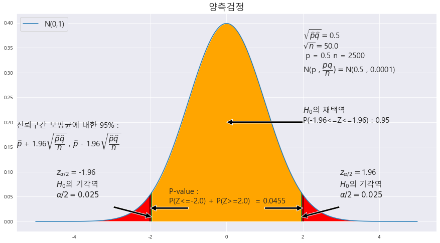
H_0 : p = 0.5(양측 검정)
p-value : 0.0455
alpha : 0.05
p-value < alpha ==> 0.0455 > 0.05 ==> 귀무가설 H_0 : p = 0.5는 기각한다. 즉 , 찬성율이 0.5가 된다는 주장이 틀렸다.
2> 1000명을 상대로 여론조사를 실시하여 520명이 이 정책에 찬성하였다.
x = np.arange(-5,5 , .001)

fig = plt.figure(figsize=(15,8))
ax = sns.lineplot(x , stats.norm.pdf(x, loc=0 , scale =1)) #정의역 범위 , 평균 = 0 , 표준편차 =1 인 정규분포 플롯

# trust = 95 #신뢰도

ax.set_title('양측검정' ,fontsize = 18)
RATIO = round(520/1000 , 4)
n = 1000
MEANS = 0.5
STDS = round(math.sqrt((MEANS * (1-MEANS) / n)),4)


#==========================================귀무가설 기각과 채택 ====================================================
trust = 95 #신뢰도_유의수준

t_1  = round(scipy.stats.norm.ppf(1 - (1-(trust/100))/2) ,3 )


ax.fill_between(x, stats.norm.pdf(x, loc=0 , scale =1) , 0 , where = (x<=t_1) & (x>=-t_1) , facecolor = 'orange') # x값 , y값 , 0 , x<=0 인곳 , 색깔
area = scipy.stats.norm.cdf(t_1) - scipy.stats.norm.cdf(-t_1)

plt.annotate('' , xy=(0, .2), xytext=(2 , .2)  , arrowprops = dict(facecolor = 'black'))
ax.text(2 , .2, r'$H_{0}$의 채택역' +f'\nP({-t_1}<=Z<={t_1}) : {round(area,4)}',fontsize=15)

annotate_len = stats.norm.pdf(t_1, loc=0 , scale =1) /2
ax.vlines(x= t_1, ymin= 0 , ymax= stats.norm.pdf(t_1, loc=0 , scale =1) , color = 'green' , linestyle ='solid' , label ='{}'.format(2))
ax.vlines(x= -t_1, ymin= 0 , ymax= stats.norm.pdf(-t_1, loc=0 , scale =1) , color = 'green' , linestyle ='solid' , label ='{}'.format(2))
area = round((1-area)/2 ,3)
ax.text(1 + t_1 , annotate_len+0.02 , r'$z_{\alpha/2} = $' + f'{t_1}\n' + r'$H_{0}$의 기각역' + f'\n'+ r'$\alpha/2 = {%.3f}$' % area,fontsize=15)
ax.text(-2.5 -t_1 , annotate_len+0.02 , r'$z_{\alpha/2} = $' + f'{-t_1}\n' + r'$H_{0}$의 기각역' + f'\n'+ r'$\alpha/2 = {%.3f}$' % area,fontsize=15)


plt.annotate('' , xy=(t_1, annotate_len-0.02), xytext=(t_1+ 1 , annotate_len)  , arrowprops = dict(facecolor = 'black'))
plt.annotate('' , xy=(-t_1, annotate_len-0.02), xytext=(-1-t_1 , annotate_len)  , arrowprops = dict(facecolor = 'black'))


ax.text(-5.5 , .15, f'신뢰구간 모평균에 대한 {trust}% : \n' + r'$\widehat{p}$' +f' + {t_1}' + r'$\sqrt{\dfrac{\widehat{p}\widehat{q}}{n}}$' +' , '+ r'$\widehat{p}$' +f' - {t_1}' + r'$\sqrt{\dfrac{\widehat{p}\widehat{q}}{n}}$',fontsize=15)


# ax.text(-5.5 , .25,  r'신뢰구간 L = $2*{%.3f}\dfrac{\sigma}{\sqrt{n}} $' % t_1 ,fontsize=15)
#
# ax.text(-5.5 , .3,  r'오차한계 = ${%.3f}\dfrac{\sigma}{\sqrt{n}} $' % t_1,fontsize=15)


#============================================표본평균의 정규분포화 =========================================================

z_1 = round((RATIO-MEANS)/STDS,4)
print(z_1)
z_1 = abs(z_1)
# # z_2 = round((34.5 - 35) / math.sqrt(5.5**2 / 25) , 2)
# z_1 = round(scipy.stats.norm.ppf(1 - (1-(trust/100))/2) ,3 )

ax.fill_between(x, stats.norm.pdf(x, loc=0 , scale =1) , 0 , where = (x<=-z_1) | (x>=z_1) , facecolor = 'skyblue') # x값 , y값 , 0 , x<=0 인곳 , 색깔
ax.fill_between(x, stats.norm.pdf(x, loc=0 , scale =1) , 0 , where = (x>=t_1) | (x<=-t_1) , facecolor = 'red') # x값 , y값 , 0 , x<=0 인곳 , 색깔
area = scipy.stats.norm.cdf(-z_1) + 1 - scipy.stats.norm.cdf(z_1)


ax.vlines(x= z_1, ymin= 0 , ymax= stats.norm.pdf(z_1, loc=0 , scale =1) , color = 'black' , linestyle ='solid' , label ='{}'.format(2))
ax.vlines(x= -z_1, ymin= 0 , ymax= stats.norm.pdf(-z_1, loc=0 , scale =1) , color = 'black' , linestyle ='solid' , label ='{}'.format(2))

annotate_len = stats.norm.pdf(z_1, loc=0 , scale =1) /2
plt.annotate('' , xy=(z_1, annotate_len), xytext=(z_1- 1 , annotate_len)  , arrowprops = dict(facecolor = 'black'))
plt.annotate('' , xy=(-z_1, annotate_len), xytext=(1-z_1 , annotate_len)  , arrowprops = dict(facecolor = 'black'))
ax.text(-1.5 , annotate_len+0.01 , f'P-value : \nP(Z<={-z_1}) + P(Z>={z_1})  = {round(area,4)}',fontsize=15)
# ax.text(0 , annotate_len+0.01 ,f'P(Z>={-z_1})',fontsize=15)


ax.text(2 , .3,  r'$\sqrt{\widehat{p}\widehat{q}} = $' + f'{round(math.sqrt(RATIO * (1-RATIO)),3)}\n'  + r'$\sqrt{n} = $' + f'{round(math.sqrt(n),2)} \n p = {MEANS} n = {n} \n' + r'N(p , ' + r'$\dfrac{pq}{n}) = $' + f'N({MEANS} , {round(MEANS*(1-MEANS)/ n ,8)})',fontsize=15)


b= 'N(0,1)'

plt.legend([b] , fontsize = 15 , loc='upper left')

H_0 : p = 0.5(양측 검정)
p-value : 0.2056
alpha : 0.05
p-value > alpha ==> 0.2056 > 0.05 ==> 귀무가설 H_0 : p = 0.5는 채택한다. 즉 , 찬성율이 0.5가 된다는 주장이 맞았다.
13. 한 포털 사이트는 우리나라 20세 이상의 성인들 중에서 인터넷 신문을 이용하는 사람의 비율이 54.5%를 초과한다고 하였다. 이를 알아보기 위하여 427명을 임의로 선정하여 인터넷 신문의 이용 여부를 조사한 결과 256명이 인터넷 신문을 이용한다고 응답하였다. 이 자료를 근거로 p-value 값을 구하여 인터넷 신문의 이용률이 54.5%를 초과하는지 유의수준 5%에서 조사하라
|X = 256/427
n = 427
trust = 95
H_0 : p <= 0.545(상단측 검정)
x = np.arange(-5,5 , .001)

fig = plt.figure(figsize=(15,8))
ax = sns.lineplot(x , stats.norm.pdf(x, loc=0 , scale =1)) #정의역 범위 , 평균 = 0 , 표준편차 =1 인 정규분포 플롯

# trust = 95 #신뢰도

ax.set_title('상단측검정' ,fontsize = 18)
RATIO = round(256/427 , 4)
n = 427
MEANS = 0.545
STDS = round(math.sqrt((MEANS * (1-MEANS) / n)),4)


#==========================================귀무가설 기각과 채택 ====================================================
trust = 95 #신뢰도_유의수준

t_1  = round(scipy.stats.norm.ppf(1 - (1-(trust/100))/2) ,3 )


ax.fill_between(x, stats.norm.pdf(x, loc=0 , scale =1) , 0 , where = (x<=t_1)  , facecolor = 'orange') # x값 , y값 , 0 , x<=0 인곳 , 색깔
area = scipy.stats.norm.cdf(t_1) - scipy.stats.norm.cdf(-t_1)

plt.annotate('' , xy=(0, .2), xytext=(2 , .2)  , arrowprops = dict(facecolor = 'black'))
ax.text(2 , .2, r'$H_{0}$의 채택역' +f'\nP(Z<={t_1}) : {round(area,4)}',fontsize=15)

annotate_len = stats.norm.pdf(t_1, loc=0 , scale =1) /2
ax.vlines(x= t_1, ymin= 0 , ymax= stats.norm.pdf(t_1, loc=0 , scale =1) , color = 'green' , linestyle ='solid' , label ='{}'.format(2))
# ax.vlines(x= -t_1, ymin= 0 , ymax= stats.norm.pdf(-t_1, loc=0 , scale =1) , color = 'green' , linestyle ='solid' , label ='{}'.format(2))
area = round((1-area),2)
ax.text(1 + t_1 , annotate_len+0.02 , r'$z_{\alpha} = $' + f'{t_1}\n' + r'$H_{0}$의 기각역' + f'\n'+ r'$\alpha = {%.3f}$' % area,fontsize=15)
# ax.text(-2.5 -t_1 , annotate_len+0.02 , r'$z_{\alpha/2} = $' + f'{-t_1}\n' + r'$H_{0}$의 기각역' + f'\n'+ r'$\alpha/2 = {%.3f}$' % area,fontsize=15)


plt.annotate('' , xy=(t_1, annotate_len-0.02), xytext=(t_1+ 1 , annotate_len)  , arrowprops = dict(facecolor = 'black'))
# plt.annotate('' , xy=(-t_1, annotate_len-0.02), xytext=(-1-t_1 , annotate_len)  , arrowprops = dict(facecolor = 'black'))


ax.text(-5.5 , .15, f'신뢰구간 모평균에 대한 {trust}% : \n' + r'$\widehat{p}$' +f' + {t_1}' + r'$\sqrt{\dfrac{\widehat{p}\widehat{q}}{n}}$' +' , '+ r'$\widehat{p}$' +f' - {t_1}' + r'$\sqrt{\dfrac{\widehat{p}\widehat{q}}{n}}$',fontsize=15)


# ax.text(-5.5 , .25,  r'신뢰구간 L = $2*{%.3f}\dfrac{\sigma}{\sqrt{n}} $' % t_1 ,fontsize=15)
#
# ax.text(-5.5 , .3,  r'오차한계 = ${%.3f}\dfrac{\sigma}{\sqrt{n}} $' % t_1,fontsize=15)


#============================================표본평균의 정규분포화 =========================================================

z_1 = round((RATIO-MEANS)/STDS,4)
print(z_1)
z_1 = abs(z_1)
# # z_2 = round((34.5 - 35) / math.sqrt(5.5**2 / 25) , 2)
# z_1 = round(scipy.stats.norm.ppf(1 - (1-(trust/100))/2) ,3 )

ax.fill_between(x, stats.norm.pdf(x, loc=0 , scale =1) , 0 , where =  (x>=z_1) , facecolor = 'skyblue') # x값 , y값 , 0 , x<=0 인곳 , 색깔
ax.fill_between(x, stats.norm.pdf(x, loc=0 , scale =1) , 0 , where = (x>=t_1)  , facecolor = 'red') # x값 , y값 , 0 , x<=0 인곳 , 색깔
area = 1 - scipy.stats.norm.cdf(z_1)


ax.vlines(x= z_1, ymin= 0 , ymax= stats.norm.pdf(z_1, loc=0 , scale =1) , color = 'black' , linestyle ='solid' , label ='{}'.format(2))
# ax.vlines(x= -z_1, ymin= 0 , ymax= stats.norm.pdf(-z_1, loc=0 , scale =1) , color = 'black' , linestyle ='solid' , label ='{}'.format(2))

annotate_len = stats.norm.pdf(z_1, loc=0 , scale =1) /2
plt.annotate('' , xy=(z_1, annotate_len), xytext=(z_1- 1 , annotate_len)  , arrowprops = dict(facecolor = 'black'))
# plt.annotate('' , xy=(-z_1, annotate_len), xytext=(1-z_1 , annotate_len)  , arrowprops = dict(facecolor = 'black'))
ax.text(-1.5 , annotate_len+0.01 , f'P-value : \nP(Z>={z_1})  = {round(area,4)}',fontsize=15)
# ax.text(0 , annotate_len+0.01 ,f'P(Z>={-z_1})',fontsize=15)


ax.text(2 , .3,  r'$\sqrt{\widehat{p}\widehat{q}} = $' + f'{round(math.sqrt(RATIO * (1-RATIO)),3)}\n'  + r'$\sqrt{n} = $' + f'{round(math.sqrt(n),2)} \n p = {MEANS} n = {n} \n' + r'N(p , ' + r'$\dfrac{pq}{n}) = $' + f'N({MEANS} , {round(MEANS*(1-MEANS)/ n ,8)})',fontsize=15)


b= 'N(0,1)'

plt.legend([b] , fontsize = 15 , loc='upper left')

H_0 : p <= 0.545(상단측 검정)
p-value : 0.0119
alpha : 0.05
p-value < alpha ==> 0.0119 < 0.05 ==> 귀무가설 H_0 : p <= 0.545 는 기각한다. 즉 , 인터넷 신문의 이용률이 54.5%를 초과한다.
14. 어느 지역에 거주하는 외국인을 상대로 조사한 보고서에 따르면, 한국인을 친근하게 느낀다고 응답한 비율이 34.4%를 넘지 않는다고 한다. 이것을 알아보기 위하여 그 지역에 거주한느 외국인 450명을 조사한 결과, 139명이 친근하게 느낀다고 응답하였다. 이 자료를 근거로 p-value 값을 구하여 보고서의 내용에 대하여 유의수준 5%에서 조사하라.
|X = 139/450
n = 450
p = 0.344
H_0 : p >= 0.344(하단측 검정)
x = np.arange(-5,5 , .001)

fig = plt.figure(figsize=(15,8))
ax = sns.lineplot(x , stats.norm.pdf(x, loc=0 , scale =1)) #정의역 범위 , 평균 = 0 , 표준편차 =1 인 정규분포 플롯

# trust = 95 #신뢰도

ax.set_title('하단측검정' ,fontsize = 18)
RATIO = round(139/450 , 4)
n = 450
MEANS = 0.344
STDS = round(math.sqrt((MEANS * (1-MEANS) / n)),4)


#==========================================귀무가설 기각과 채택 ====================================================
trust = 95 #신뢰도_유의수준

t_1  = round(scipy.stats.norm.ppf(1 - (1-(trust/100))/2) ,3 )


ax.fill_between(x, stats.norm.pdf(x, loc=0 , scale =1) , 0 , where = (x>=-t_1) , facecolor = 'orange') # x값 , y값 , 0 , x<=0 인곳 , 색깔
area = scipy.stats.norm.cdf(t_1) - scipy.stats.norm.cdf(-t_1)

plt.annotate('' , xy=(0, .2), xytext=(2 , .2)  , arrowprops = dict(facecolor = 'black'))
ax.text(2 , .2, r'$H_{0}$의 채택역' +f'\nP({-t_1}<=Z) : {round(area,4)}',fontsize=15)

annotate_len = stats.norm.pdf(t_1, loc=0 , scale =1) /2
# ax.vlines(x= t_1, ymin= 0 , ymax= stats.norm.pdf(t_1, loc=0 , scale =1) , color = 'green' , linestyle ='solid' , label ='{}'.format(2))
ax.vlines(x= -t_1, ymin= 0 , ymax= stats.norm.pdf(-t_1, loc=0 , scale =1) , color = 'green' , linestyle ='solid' , label ='{}'.format(2))
area = round((1-area) ,3)
# ax.text(1 + t_1 , annotate_len+0.02 , r'$z_{\alpha/2} = $' + f'{t_1}\n' + r'$H_{0}$의 기각역' + f'\n'+ r'$\alpha/2 = {%.3f}$' % area,fontsize=15)
ax.text(-2.5 -t_1 , annotate_len+0.02 , r'$z_{\alpha} = $' + f'{-t_1}\n' + r'$H_{0}$의 기각역' + f'\n'+ r'$\alpha = {%.3f}$' % area,fontsize=15)


# plt.annotate('' , xy=(t_1, annotate_len-0.02), xytext=(t_1+ 1 , annotate_len)  , arrowprops = dict(facecolor = 'black'))
plt.annotate('' , xy=(-t_1, annotate_len-0.02), xytext=(-1-t_1 , annotate_len)  , arrowprops = dict(facecolor = 'black'))


ax.text(-5.5 , .15, f'신뢰구간 모평균에 대한 {trust}% : \n' + r'$\widehat{p}$' +f' + {t_1}' + r'$\sqrt{\dfrac{\widehat{p}\widehat{q}}{n}}$' +' , '+ r'$\widehat{p}$' +f' - {t_1}' + r'$\sqrt{\dfrac{\widehat{p}\widehat{q}}{n}}$',fontsize=15)


# ax.text(-5.5 , .25,  r'신뢰구간 L = $2*{%.3f}\dfrac{\sigma}{\sqrt{n}} $' % t_1 ,fontsize=15)
#
# ax.text(-5.5 , .3,  r'오차한계 = ${%.3f}\dfrac{\sigma}{\sqrt{n}} $' % t_1,fontsize=15)


#============================================표본평균의 정규분포화 =========================================================

z_1 = round((RATIO-MEANS)/STDS,4)
print(z_1)
z_1 = abs(z_1)
# # z_2 = round((34.5 - 35) / math.sqrt(5.5**2 / 25) , 2)
# z_1 = round(scipy.stats.norm.ppf(1 - (1-(trust/100))/2) ,3 )

ax.fill_between(x, stats.norm.pdf(x, loc=0 , scale =1) , 0 , where = (x<=-z_1) , facecolor = 'skyblue') # x값 , y값 , 0 , x<=0 인곳 , 색깔
ax.fill_between(x, stats.norm.pdf(x, loc=0 , scale =1) , 0 , where =  (x<=-t_1) , facecolor = 'red') # x값 , y값 , 0 , x<=0 인곳 , 색깔
area = scipy.stats.norm.cdf(-z_1)


# ax.vlines(x= z_1, ymin= 0 , ymax= stats.norm.pdf(z_1, loc=0 , scale =1) , color = 'black' , linestyle ='solid' , label ='{}'.format(2))
ax.vlines(x= -z_1, ymin= 0 , ymax= stats.norm.pdf(-z_1, loc=0 , scale =1) , color = 'black' , linestyle ='solid' , label ='{}'.format(2))

annotate_len = stats.norm.pdf(z_1, loc=0 , scale =1) /2
# plt.annotate('' , xy=(z_1, annotate_len), xytext=(z_1- 1 , annotate_len)  , arrowprops = dict(facecolor = 'black'))
plt.annotate('' , xy=(-z_1, annotate_len), xytext=(1-z_1 , annotate_len)  , arrowprops = dict(facecolor = 'black'))
ax.text(-1.5 , annotate_len+0.01 , f'P-value : \nP(Z<={-z_1})  = {round(area,4)}',fontsize=15)
# ax.text(0 , annotate_len+0.01 ,f'P(Z>={-z_1})',fontsize=15)


ax.text(2 , .3,  r'$\sqrt{\widehat{p}\widehat{q}} = $' + f'{round(math.sqrt(RATIO * (1-RATIO)),3)}\n'  + r'$\sqrt{n} = $' + f'{round(math.sqrt(n),2)} \n p = {MEANS} n = {n} \n' + r'N(p , ' + r'$\dfrac{pq}{n}) = $' + f'N({MEANS} , {round(MEANS*(1-MEANS)/ n ,8)})',fontsize=15)


b= 'N(0,1)'

plt.legend([b] , fontsize = 15 , loc='upper left')

H_0 : p >= 0.344(상단측 검정)
p-value : 0.0586
alpha : 0.05
p-value > alpha ==> 0.0586 < 0.05 ==> 귀무가설 H_0 : p >= 0.344 는 채택한다. 즉 , 외국인중 한국인을 친근하다고 느끼는 비율은 34.4%를 넘는다.