★카이제곱분포★모분산에 대한 소표본 추론★기초통계학-[소표본 추론-06]
1. 모분산에 대한 소표본 추론
==> 정규모집단의 모분산과 모표준편차에 대한 구간추정 및 가설검정 방법
https://knowallworld.tistory.com/321
★종합선물세트★F-분포(표본분산의 비 이용!)★표본평균의 차에 따른 확률분포!★합동표본분산
29. 두 정규모집단 A와 B의 모분산은 동일하고, 평균은 각각 뮤_1 = 700 , 뮤_2 = 680이라 한다. 두 모집단으로 부터 표본을 추출하여 A 표본 [n = 17 , |x = 704 , s_1 = 39.25] , B표본 [m = 10 , |y = 675 , s_2 = 43.75] h
knowallworld.tistory.com
https://knowallworld.tistory.com/305
★표본분산 S**2 , 관찰 표본분산 s_0**2★카이제곱분포표★모분산의 표본분포★기초통계학-[모집
1. 모분산의 표본분포 정규모집단 N(뮤 , 모분산) 으로부터 크기 n인 표본을 선정할 때 표본분산 ==> 표본분산 S**2에 대한 표본분포는 X**2-통계량 V에 대하여 자유도가 n-1인 카이제곱분포이다. https:
knowallworld.tistory.com

EX-01) 어느 제약회사에서 생산되는 캡슐 감기약의 무게에 대한 분산을 알아보기 위하여 시중에서 판매되는 감기약 16개를 수거하여 무게를 측정한 결과 다음과 같았다. 이 자료를 이용하여 다음을 구하라.
X = np.arange(0,30 , .01)

fig = plt.figure(figsize=(20,12))


A = '4.23 4.26 4.26 4.24 4.27 4.23 4.19 4.27 4.21 4.25 4.23 4.29 4.30 4.24 4.20 4.24'
A= list(map(float , A.split(' ')))

Vars = np.var(A , ddof=1)

dof_2 = [len(A)-1] #자유도

trust = 95
trust = round((1- trust/100)/2,3)

n = len(A)

STDS = math.sqrt(Vars)
ax = sns.lineplot(x = X , y=scipy.stats.chi2(dof_2).pdf(X) )
X_r =  scipy.stats.chi2(dof_2).ppf(1-trust)
X_l = scipy.stats.chi2(dof_2).ppf(trust)
# t_r = round( (x_0 - (0)) / (math.sqrt(33.463) * math.sqrt(1/16 + 1/16)), 3)
print(X_r)


ax.fill_between(X, scipy.stats.chi2(dof_2).pdf(X) , 0 , where = (X>=X_r) | (X<=X_l) , facecolor = 'skyblue') # x값 , y값 , 0 , X조건 인곳 , 색깔
ax.fill_between(X, scipy.stats.chi2(dof_2).pdf(X) , 0 , where = (X<=X_r) & (X>=X_l) , facecolor = 'orange')


ax.vlines(x = X_r ,ymin=0 , ymax= scipy.stats.chi2(dof_2).pdf(X_r) , colors = 'black')
ax.vlines(x = X_l ,ymin=0 , ymax= scipy.stats.chi2(dof_2).pdf(X_l) , colors = 'black')
plt.annotate('' , xy=(X_r + 2, .001), xytext=(28 , .01)  , arrowprops = dict(facecolor = 'black'))
plt.annotate('' , xy=(X_l - 2, .001), xytext=(2 , .01)  , arrowprops = dict(facecolor = 'black'))
area = 1- scipy.stats.chi2(dof_2).cdf(X_r)
ax.text(X_r , .011, r'$\chi^2_{%.3f}$' % trust + f'= {area}',fontsize=15)
ax.text(X_l- 5 , .011, r'$\chi^2_{%.3f}$' % (1-trust) + f'= {area}',fontsize=15)


ax.text(18 , 0.07 , f'n< 10에 대한 신뢰구간\n' + r'$(e_{%d})= \left(\dfrac{(n-1)s^{2}}{X^2_{\alpha/2 , n-1}} ,\dfrac{(n-1)s^{2}}{X^2_{-(\alpha/2) , n-1}} \right)$' % ((1- (trust*2))*100) + f'\n = ({round(float((n-1) * STDS**2 / X_r),5)} , {round(float((n-1) * STDS**2 / X_l),5)})' , fontsize = 16)
ax.text(18 , 0.05 ,f'n>= 10에 대한 신뢰구간\n' +  r'신뢰구간$(e_{%d}) = \left(s\sqrt{\dfrac{(n-1)}{X^2_{\alpha/2 , n-1}}} ,s\sqrt{\dfrac{(n-1)}{X^2_{-(\alpha/2) , n-1}}} \right)$' % ((1- (trust*2))*100) + f'\n = ({round(math.sqrt((n-1) * STDS**2 / X_r),4)} , {round(math.sqrt((n-1) * STDS**2 / X_l),4)})' , fontsize = 16)
ax.text(0 , 0.07 , r'카이제곱분포(V) = $\left(\dfrac{(n-1)s^{2}}{\sigma^{2}}\right)$' + f'\n n = {n}\n s = {STDS}' , fontsize = 16)


ax.text(X_l + 0.4 , scipy.stats.chi2(dof_2).pdf(X_l)/2 , r'$\chi^2_L= {%.4f}$' % X_l  , fontsize = 13)
ax.text(X_r - 3 , scipy.stats.chi2(dof_2).pdf(X_r)/2 , r'$\chi^2_R= {%.4f}$' % X_r   , fontsize = 13)


b = ['t-(n={})'.format(i) for i in dof_2]
plt.legend(b , fontsize = 15)
==> 모분산에 의한 신뢰구간 ==> (0.0005 , 0.0022)
==> 모표준편차에 의한 신뢰구간 ==> (0.0224 , 0.0469)
EX-02) 제주도에서 여름 휴가를 보내기 위해 무작위로 동일한 규모의 펜션 사용료를 조사한 결과 다음과 같았다. 물음에 답하라.
X = np.arange(0,30 , .01)

fig = plt.figure(figsize=(20,12))


A = '12.5 11.5 6.0 5.5 15.5 11.5 10.5 17.5 10.0 9.5 13.5 8.5 11.5 15.5'
A= list(map(float , A.split(' ')))

Vars = np.var(A , ddof=1)

dof_2 = [len(A)-1] #자유도

trust = 95
trust = round((1- trust/100)/2,3)

n = len(A)

STDS = math.sqrt(Vars)
ax = sns.lineplot(x = X , y=scipy.stats.chi2(dof_2).pdf(X) )
X_r =  scipy.stats.chi2(dof_2).ppf(1-trust)
X_l = scipy.stats.chi2(dof_2).ppf(trust)
# t_r = round( (x_0 - (0)) / (math.sqrt(33.463) * math.sqrt(1/16 + 1/16)), 3)
print(X_r)


ax.fill_between(X, scipy.stats.chi2(dof_2).pdf(X) , 0 , where = (X>=X_r) | (X<=X_l) , facecolor = 'skyblue') # x값 , y값 , 0 , X조건 인곳 , 색깔
ax.fill_between(X, scipy.stats.chi2(dof_2).pdf(X) , 0 , where = (X<=X_r) & (X>=X_l) , facecolor = 'orange')


ax.vlines(x = X_r ,ymin=0 , ymax= scipy.stats.chi2(dof_2).pdf(X_r) , colors = 'black')
ax.vlines(x = X_l ,ymin=0 , ymax= scipy.stats.chi2(dof_2).pdf(X_l) , colors = 'black')
plt.annotate('' , xy=(X_r + 2, .001), xytext=(28 , .01)  , arrowprops = dict(facecolor = 'black'))
plt.annotate('' , xy=(X_l - 2, .001), xytext=(2 , .01)  , arrowprops = dict(facecolor = 'black'))
area = 1- scipy.stats.chi2(dof_2).cdf(X_r)
ax.text(X_r , .011, r'$\chi^2_{%.3f}$' % trust + f'= {area}',fontsize=15)
ax.text(X_l- 5 , .011, r'$\chi^2_{%.3f}$' % (1-trust) + f'= {area}',fontsize=15)


ax.text(18 , 0.07 , f'n< 10에 대한 신뢰구간\n' + r'$(e_{%d})= \left(\dfrac{(n-1)s^{2}}{X^2_{\alpha/2 , n-1}} ,\dfrac{(n-1)s^{2}}{X^2_{-(\alpha/2) , n-1}} \right)$' % ((1- (trust*2))*100) + f'\n = ({round(float((n-1) * STDS**2 / X_r),5)} , {round(float((n-1) * STDS**2 / X_l),5)})' , fontsize = 16)
ax.text(18 , 0.05 ,f'n>= 10에 대한 신뢰구간\n' +  r'신뢰구간$(e_{%d}) = \left(s\sqrt{\dfrac{(n-1)}{X^2_{\alpha/2 , n-1}}} ,s\sqrt{\dfrac{(n-1)}{X^2_{-(\alpha/2) , n-1}}} \right)$' % ((1- (trust*2))*100) + f'\n = ({round(math.sqrt((n-1) * STDS**2 / X_r),4)} , {round(math.sqrt((n-1) * STDS**2 / X_l),4)})' , fontsize = 16)
ax.text(0 , 0.07 , r'카이제곱분포(V) = $\left(\dfrac{(n-1)s^{2}}{\sigma^{2}}\right)$' + f'\n n = {n}\n s = {STDS}' , fontsize = 16)


ax.text(X_l + 0.4 , scipy.stats.chi2(dof_2).pdf(X_l)/2 , r'$\chi^2_L= {%.4f}$' % X_l  , fontsize = 13)
ax.text(X_r - 3 , scipy.stats.chi2(dof_2).pdf(X_r)/2 , r'$\chi^2_R= {%.4f}$' % X_r   , fontsize = 13)


b = ['t-(n={})'.format(i) for i in dof_2]
plt.legend(b , fontsize = 15)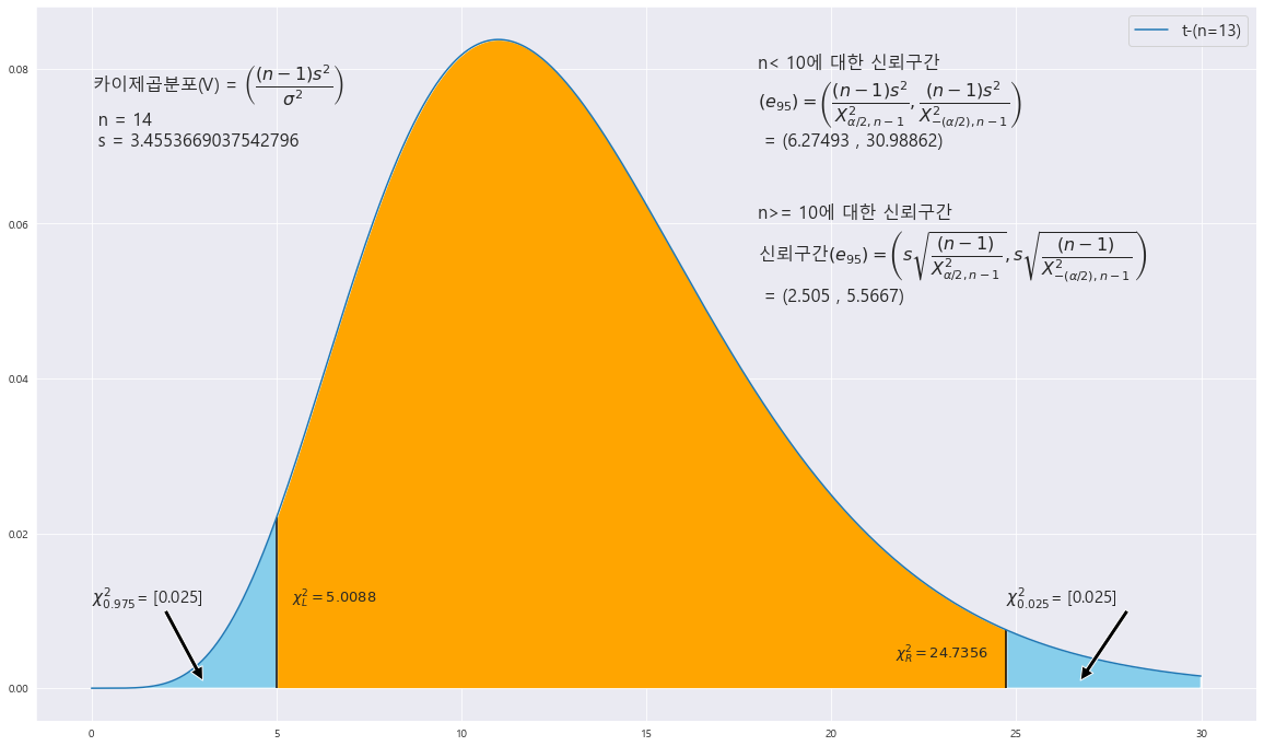
==> 모분산에 의한 신뢰구간 ==> (6.27493 , 30.98862)
==> 모표준편차에 의한 신뢰구간 ==> (2.505 , 5.5667)
'기초통계 > 소표본 추론' 카테고리의 다른 글
| ★모분산 비에 대한 소표본 추론★기초통계학-[소표본 추론-08] (0) | 2023.01.18 |
|---|---|
| ★카이제곱분포★모분산에 대한 가설검정★양측검정★상단측,하단측검정★기초통계학-[소표본 추론-07] (0) | 2023.01.18 |
| ★쌍체 t-검정★기초통계학-[소표본 추론-05] (0) | 2023.01.17 |
| ★모평균의 차에 대한 소표본 가설검정★기초통계학-[소표본 추론-04] (0) | 2023.01.17 |
| ★t-분포의 합동표본분산 구하는거 기억하기★모평균 차에 대한 소표본 추정★기초통계학-[소표본 추론-03] (0) | 2023.01.17 |