https://knowallworld.tistory.com/302
★모분산을 모를땐 t-분포!★stats.norm.cdf()★모분산을 알때/모를때 표본평균의 표본분포★일표본
1. 표본평균의 표본분포(모분산을 아는 경우) ==> 표본평균에 대한 표본분포는 정규분포를 따른다. EX-01) 모평균 100 , 모분산 9인 정규모집단으로부터 크기 25인 표본을 임의로 추출 1> 표본평균 |X
knowallworld.tistory.com

1. t-분포에 대한 양측검정
==> 양측검정의 귀무가설은 '='
EX-01) 리필용 플라스틱 샴푸 용기를 만드는 한 제조 회사가 국내 최대 용량인 1100ml 의 용기를 생산했다고 광고한다. 이를 확인하기 위해서 18개의 용기를 임의로 수거하여 샴푸의 용량을 조사한 결과 다음과 같았다. 이 자료를 이용하여 샴푸 용기 제조 회사의 주장에 대해 유의수준 5%에서 조사하라.
A = "1073 1067 1103 1122 1057 1096 1057 1053 1089 1102 1100 1091 1053 1138 1063 1120 1077 1091"
A = list(map(int, A.split(' ')))
X = np.arange(-5,5 , .01)
fig = plt.figure(figsize=(15,8))
A = "1073 1067 1103 1122 1057 1096 1057 1053 1089 1102 1100 1091 1053 1138 1063 1120 1077 1091"
A = list(map(int, A.split(' ')))
MEANS = round(np.mean(A),4)
STDS = round(np.std(A , ddof =1 ) , 4)
MO_MEAN = 1100
n = len(A) #표본개수
dof_2 = [n-1] #자유도c
ax = sns.lineplot(x = X , y=scipy.stats.t(dof_2).pdf(X) )
trust = 95 #신뢰도
trust = round( (1- trust/100)/2 , 4)
t_r = scipy.stats.t(dof_2).ppf(1- trust)
print(t_r)
t_l = scipy.stats.t(dof_2).ppf(trust)
print(t_l)
E = round(float(t_r * STDS / math.sqrt(n)),4)
# =========================================================
ax.fill_between(X, scipy.stats.t(dof_2).pdf(X) , 0 , where = (X<t_r) & (X>t_l) , facecolor = 'orange') # x값 , y값 , 0 , X조건 인곳 , 색깔
area = round(float(scipy.stats.t(dof_2).cdf(t_r) - scipy.stats.t(dof_2).cdf(t_l)),4)
plt.annotate('' , xy=(0, .2), xytext=(-2.5 , .25) , arrowprops = dict(facecolor = 'black'))
ax.text(-4.6 , .32, f'평균(MEANS) = {MEANS}\n' +f' n = {n} \n 표준편차(s) = {STDS}\n' +r'오차한계 $e_{95\% } = t_{\dfrac{\alpha}{2}}*\dfrac{s}{\sqrt{n}}$'+f'= {E}',fontsize=15)
plt.annotate('' , xy=(0, .25), xytext=(1.5 , .25) , arrowprops = dict(facecolor = 'black'))
ax.text(1.6 , .25, r'$P(t_{%.3f}<T<t_{%.3f})$' % (trust , 1-trust) + f'= {area}\n' + r'신뢰구간 = (MEANS -$e_{\alpha}$ , MEANS + $e_{\alpha}$)' +f'\n' + r' = $({%.4f} - {%.4f} , {%.4f} + {%.4f})$' % (MEANS, E , MEANS , E) +f'\n' +r'$ = ({%.4f} , {%.4f})$' % (MEANS-E , MEANS+E) ,fontsize=15)
ax.vlines(x = t_r ,ymin=0 , ymax= scipy.stats.t(dof_2).pdf(t_r) , colors = 'black')
ax.vlines(x = t_l ,ymin=0 , ymax= scipy.stats.t(dof_2).pdf(t_l) , colors = 'black')
plt.annotate('' , xy=(t_r, .007), xytext=(2.5 , .1) , arrowprops = dict(facecolor = 'black'))
plt.annotate('' , xy=(t_l, .007), xytext=(-3.5 , .1) , arrowprops = dict(facecolor = 'black'))
ax.text(1.71 , .13, r'$t_{\dfrac{\alpha}{2}} = {%.4f}$' % t_r + '\n' +r'$\dfrac{\alpha}{2}$ =' + f'{round(float(1- scipy.stats.t(dof_2).cdf(t_r)),3)}',fontsize=15)
ax.text(-3.71 , .13, r'$t_{\dfrac{\alpha}{2}} = {%.4f}$' % t_l + '\n' +r'$\dfrac{\alpha}{2}$ =' +f'{round(float(scipy.stats.t(dof_2).cdf(t_l)),3)}',fontsize=15)
ax.text(t_r - 1 , 0.02 , r'$t_r$' + f'= {t_r}' , fontsize = 13)
ax.text(t_l + .2 , 0.02 , r'$t_l$' + f'= {t_l}' , fontsize = 13)
#==================================== 가설 검정 ==========================================
t_1 = round((MEANS - MO_MEAN)/ (STDS / math.sqrt(n)),4)
print(t_1)
t_1 = abs(t_1)
area = round(float(scipy.stats.t(dof_2).cdf(-t_1) + 1 - (scipy.stats.t(dof_2).cdf(t_1))),4)
ax.fill_between(X, scipy.stats.t(dof_2).pdf(X) , 0 , where = (X>=t_1) | (X<=-t_1) , facecolor = 'skyblue') # x값 , y값 , 0 , X조건 인곳 , 색깔
ax.fill_between(X, scipy.stats.t(dof_2).pdf(X) , 0 , where = (X>=t_r) | (X<=-t_r) , facecolor = 'red') # x값 , y값 , 0 , X조건 인곳 , 색깔
ax.vlines(x= t_1, ymin= 0 , ymax= stats.t(dof_2).pdf(t_1) , color = 'green' , linestyle ='solid' , label ='{}'.format(2))
ax.vlines(x= -t_1, ymin= 0 , ymax= stats.t(dof_2).pdf(-t_1) , color = 'green' , linestyle ='solid' , label ='{}'.format(2))
annotate_len = stats.t(dof_2).pdf(t_1) /2
plt.annotate('' , xy=(t_1, annotate_len), xytext=(-t_1/2 , annotate_len) , arrowprops = dict(facecolor = 'black'))
plt.annotate('' , xy=(-t_1, annotate_len), xytext=(t_1/2 , annotate_len) , arrowprops = dict(facecolor = 'black'))
ax.text(-1.5 , annotate_len+0.03 , f'P-value : \nP(T<={-t_1}) + P(T>={t_1}) \n = {area}',fontsize=15)
mo = '모평균'
ax.text(-4.6 , .22, r'T = $\dfrac{\overline{X} - {\mu}}{\dfrac{s}{\sqrt{n}}}$' + f'= { round((MEANS - MO_MEAN)/(STDS / math.sqrt(n)),4) }' ,fontsize=15)
b = ['t-(n={})'.format(i) for i in dof_2]
plt.legend(b , fontsize = 15)
p-value : 0.0349
alpha : 0.05
p-value < alpha ==> 0.0349 > 0.05 ==> 귀무가설 H_0 : m = 1100 는 기각한다. 즉 , 유의수준 5%에서 삼퓨 용기 제조회사의 주장은 설득력이 없다.
EX-02) 어느 음료수 제조 회사에서 시판 중인 음료수의 용량이 360mL 라고 한다. 이 음료수 6개를 수거하여 용량을 측정한 결과, 평균 360.6mL, 표준편차 0.74mL 였다. 이 결과를 이용하여 유의수준 10%에서 음료수의 용량을 조사하라.
H_0 : m = 360
X = np.arange(-5,5 , .01)

fig = plt.figure(figsize=(15,8))


#
# A = "1073 1067 1103 1122 1057 1096 1057 1053 1089 1102 1100 1091 1053 1138 1063 1120 1077 1091"
# A = list(map(int, A.split(' ')))


MEANS = 360.6
STDS = 0.74
MO_MEAN = 360


n = 6 #표본개수
dof_2 = [n-1] #자유도c

ax = sns.lineplot(x = X , y=scipy.stats.t(dof_2).pdf(X) )
trust = 90 #신뢰도
trust = round( (1- trust/100)/2 , 4)
t_r =  scipy.stats.t(dof_2).ppf(1- trust)
print(t_r)
t_l = scipy.stats.t(dof_2).ppf(trust)
print(t_l)

E = round(float(t_r * STDS / math.sqrt(n)),4)


# =========================================================

ax.fill_between(X, scipy.stats.t(dof_2).pdf(X) , 0 , where = (X<t_r) & (X>t_l) , facecolor = 'orange') # x값 , y값 , 0 , X조건 인곳 , 색깔
area = round(float(scipy.stats.t(dof_2).cdf(t_r) - scipy.stats.t(dof_2).cdf(t_l)),4)


plt.annotate('' , xy=(0, .2), xytext=(-2.5 , .25)  , arrowprops = dict(facecolor = 'black'))
ax.text(-4.6 , .32, f'평균(MEANS) = {MEANS}\n'  +f' n = {n} \n 표준편차(s) = {STDS}\n' +r'오차한계 $e_{%d} = t_{\dfrac{\alpha}{2}}*\dfrac{s}{\sqrt{n}}$' % ((1-  trust*2)*100 ) +f'= {E}' ,fontsize=15)

plt.annotate('' , xy=(0, .25), xytext=(1.5 , .25)  , arrowprops = dict(facecolor = 'black'))
ax.text(1.6 , .25, r'$P(t_{%.3f}<T<t_{%.3f})$' % (trust , 1-trust) + f'= {area}\n' + r'신뢰구간 = (MEANS -$e_{\alpha}$ , MEANS + $e_{\alpha}$)' +f'\n' + r' = $({%.4f} - {%.4f} , {%.4f} + {%.4f})$' % (MEANS, E , MEANS , E)  +f'\n' +r'$ = ({%.4f} , {%.4f})$' % (MEANS-E , MEANS+E)  ,fontsize=15)

ax.vlines(x = t_r ,ymin=0 , ymax= scipy.stats.t(dof_2).pdf(t_r) , colors = 'black')
ax.vlines(x = t_l ,ymin=0 , ymax= scipy.stats.t(dof_2).pdf(t_l) , colors = 'black')


plt.annotate('' , xy=(t_r, .007), xytext=(2.5 , .1)  , arrowprops = dict(facecolor = 'black'))
plt.annotate('' , xy=(t_l, .007), xytext=(-3.5 , .1)  , arrowprops = dict(facecolor = 'black'))
ax.text(1.71 , .13, r'$t_{\dfrac{\alpha}{2}} = {%.4f}$' % t_r + '\n' +r'$\dfrac{\alpha}{2}$ =' + f'{round(float(1- scipy.stats.t(dof_2).cdf(t_r)),3)}',fontsize=15)
ax.text(-3.71 , .13, r'$t_{\dfrac{\alpha}{2}} = {%.4f}$' % t_l + '\n' +r'$\dfrac{\alpha}{2}$ =' +f'{round(float(scipy.stats.t(dof_2).cdf(t_l)),3)}',fontsize=15)

ax.text(t_r - 1 , 0.02 , r'$t_r$' + f'= {t_r}'  , fontsize = 13)
ax.text(t_l + .2 , 0.02 , r'$t_l$' + f'= {t_l}'  , fontsize = 13)


#==================================== 가설 검정 ==========================================


t_1 = round((MEANS - MO_MEAN)/ (STDS / math.sqrt(n)),4)

print(t_1)
t_1 = abs(t_1)
area = round(float(scipy.stats.t(dof_2).cdf(-t_1) + 1 - (scipy.stats.t(dof_2).cdf(t_1))),4)
ax.fill_between(X, scipy.stats.t(dof_2).pdf(X) , 0 , where = (X>=t_1) | (X<=-t_1) , facecolor = 'skyblue') # x값 , y값 , 0 , X조건 인곳 , 색깔
ax.fill_between(X, scipy.stats.t(dof_2).pdf(X) , 0 , where = (X>=t_r) | (X<=-t_r) , facecolor = 'red') # x값 , y값 , 0 , X조건 인곳 , 색깔

ax.vlines(x= t_1, ymin= 0 , ymax= stats.t(dof_2).pdf(t_1) , color = 'green' , linestyle ='solid' , label ='{}'.format(2))
ax.vlines(x= -t_1, ymin= 0 , ymax= stats.t(dof_2).pdf(-t_1) , color = 'green' , linestyle ='solid' , label ='{}'.format(2))

annotate_len = stats.t(dof_2).pdf(t_1) /2
plt.annotate('' , xy=(t_1, annotate_len), xytext=(-t_1/2 , annotate_len)  , arrowprops = dict(facecolor = 'black'))
plt.annotate('' , xy=(-t_1, annotate_len), xytext=(t_1/2 , annotate_len)  , arrowprops = dict(facecolor = 'black'))
ax.text(-1.5 , annotate_len+0.03 , f'P-value : \nP(T<={-t_1}) + P(T>={t_1}) \n = {area}',fontsize=15)

mo = '모평균'

ax.text(-4.6 , .22, r'T = $\dfrac{\overline{X} - {\mu}}{\dfrac{s}{\sqrt{n}}}$' + f'= { round((MEANS - MO_MEAN)/(STDS / math.sqrt(n)),4) }' ,fontsize=15)


b = ['t-(n={})'.format(i) for i in dof_2]
plt.legend(b , fontsize = 15)
p-value : 0.1038
alpha : 0.1
p-value > alpha ==> 0.1038 > 0.1 ==> 귀무가설 H_0 : m = 360 는 채택한다. 즉 , 유의수준 10%에서 음료수의 용량이 360mL라는 주장은 설득력이 있다.
2. t-분포에 대한 하단측검정
EX-03) 어느 타이어 제조 회사에서 생산된 타이어의 평균 수명이 10이상인지 알아보기 위하여 이 회사의 타이어 10개를 조사한 결과, 평균 9.6 , 표준편차 0.504였다. 이 자료를 이용하여 타이어의 평균 수명이 10 이상인지 유의수준 2.5%에서 조사하라.
H_0 : 평균수명 >= 10
|X = 9.6
s = 0.504
n = 10
X = np.arange(-5,5 , .01)

fig = plt.figure(figsize=(15,8))


#
# A = "1073 1067 1103 1122 1057 1096 1057 1053 1089 1102 1100 1091 1053 1138 1063 1120 1077 1091"
# A = list(map(int, A.split(' ')))


MEANS = 9.6
STDS = 0.504
MO_MEAN = 10


n = 10 #표본개수
dof_2 = [n-1] #자유도c

ax = sns.lineplot(x = X , y=scipy.stats.t(dof_2).pdf(X) )
trust = 97.5 #신뢰도
trust = round( (1- trust/100) , 4)
t_r =  scipy.stats.t(dof_2).ppf(1- trust)
print(t_r)
t_l = scipy.stats.t(dof_2).ppf(trust)
print(t_l)

E = round(float(t_r * STDS / math.sqrt(n)),4) #오차한계


ax.set_title('하단측검정' , fontsize = 15)
# =========================================================

ax.fill_between(X, scipy.stats.t(dof_2).pdf(X) , 0 , where = (X>=-t_r)  , facecolor = 'orange') # x값 , y값 , 0 , X조건 인곳 , 색깔
area = round(float(1- scipy.stats.t(dof_2).cdf(t_l)),4)


plt.annotate('' , xy=(0, .2), xytext=(-2.5 , .25)  , arrowprops = dict(facecolor = 'black'))
ax.text(-4.6 , .32, f'평균(MEANS) = {MEANS}\n'  +f' n = {n} \n 표준편차(s) = {STDS}\n' +r'오차한계 $e_{%d} = t_{{\alpha}}*\dfrac{s}{\sqrt{n}}$' % ((1-  trust)*100 ) +f'= {E}' ,fontsize=15)

plt.annotate('' , xy=(0, .25), xytext=(1.5 , .25)  , arrowprops = dict(facecolor = 'black'))
ax.text(1.6 , .25, r'$P(t_{%.3f}<T)$' % (trust) + f'= {area}\n' + r'신뢰구간 = (MEANS -$e_{\alpha}$ , MEANS + $e_{\alpha}$)' +f'\n' + r' = $({%.4f} - {%.4f} , {%.4f} + {%.4f})$' % (MEANS, E , MEANS , E)  +f'\n' +r'$ = ({%.4f} , {%.4f})$' % (MEANS-E , MEANS+E)  ,fontsize=15)

# ax.vlines(x = t_r ,ymin=0 , ymax= scipy.stats.t(dof_2).pdf(t_r) , colors = 'black')
ax.vlines(x = t_l ,ymin=0 , ymax= scipy.stats.t(dof_2).pdf(t_l) , colors = 'black')


# plt.annotate('' , xy=(t_r, .007), xytext=(2.5 , .1)  , arrowprops = dict(facecolor = 'black'))
plt.annotate('' , xy=(t_l, .007), xytext=(-3.5 , .1)  , arrowprops = dict(facecolor = 'black'))
# ax.text(1.71 , .13, r'$t_{\dfrac{\alpha}{2}} = {%.4f}$' % t_r + '\n' +r'$\dfrac{\alpha}{2}$ =' + f'{round(float(1- scipy.stats.t(dof_2).cdf(t_r)),3)}',fontsize=15)
ax.text(-3.71 , .13, r'$t_{{\alpha}} = {%.4f}$' % t_l + '\n' +r'${\alpha}$ =' +f'{round(float(scipy.stats.t(dof_2).cdf(t_l)),3)}',fontsize=15)

# ax.text(t_r - 1 , 0.02 , r'$t_r$' + f'= {t_r}'  , fontsize = 13)
ax.text(t_l + .2 , 0.02 , r'$t_l$' + f'= {t_l}'  , fontsize = 13)


#==================================== 가설 검정 ==========================================


t_1 = round((MEANS - MO_MEAN)/ (STDS / math.sqrt(n)),4)

print(t_1)
t_1 = abs(t_1)
area = round(float(scipy.stats.t(dof_2).cdf(-t_1) ),4)
ax.fill_between(X, scipy.stats.t(dof_2).pdf(X) , 0 , where =  (X<=-t_1) , facecolor = 'skyblue') # x값 , y값 , 0 , X조건 인곳 , 색깔
ax.fill_between(X, scipy.stats.t(dof_2).pdf(X) , 0 , where = (X<=t_l) , facecolor = 'red') # x값 , y값 , 0 , X조건 인곳 , 색깔

# ax.vlines(x= t_1, ymin= 0 , ymax= stats.t(dof_2).pdf(t_1) , color = 'green' , linestyle ='solid' , label ='{}'.format(2))
ax.vlines(x= -t_1, ymin= 0 , ymax= stats.t(dof_2).pdf(-t_1) , color = 'green' , linestyle ='solid' , label ='{}'.format(2))

annotate_len = stats.t(dof_2).pdf(t_1) /2
# plt.annotate('' , xy=(t_1, annotate_len), xytext=(-t_1/2 , annotate_len)  , arrowprops = dict(facecolor = 'black'))
plt.annotate('' , xy=(-t_1, annotate_len), xytext=(t_1/2 , annotate_len)  , arrowprops = dict(facecolor = 'black'))
ax.text(0.7, annotate_len+0.03 , f'P-value : \nP(T<={-t_1}) \n = {area}',fontsize=15)

mo = '모평균'

ax.text(-4.6 , .22, r'T = $\dfrac{\overline{X} - {\mu}}{\dfrac{s}{\sqrt{n}}}$' + f'= { round((MEANS - MO_MEAN)/(STDS / math.sqrt(n)),4) }' ,fontsize=15)


b = ['t-(n={})'.format(i) for i in dof_2]
plt.legend(b , fontsize = 15)
p-value : 0.0167
alpha : 0.025
p-value < alpha ==> 0.0167 > 0.025 ==> 귀무가설 H_0 : m >= 10(하단측 검정) 은 기각한다. 즉 , 유의수준 2.5%에서 타이어의 평균 수명은 10 이상의 증거가 불충분하다.
EX-04) 뼈와 치아에 가장 중요한 요소 중 하나인 칼슘의 하루 섭취량은 800 mg 이다. 차상위 계층 이하인 사람들의 하루 섭취량이 이 기준에 미치지 못하는지 알아보기 위하여 6명의 차상위 계층 이하인 사람을 임의로 선정하여 조사한 결과, 평균 774 mg , 표준편차 31.4mg 이었다. 이 자료를 이용하여 차상위 계층 이하인 사람들의 하루 칼슘 섭취량의 미달 여부를 유의수준 5%에서 조사하라.
|X = 774
s = 31.4
n = 6
H_0 : M >= 800
X = np.arange(-5,5 , .01)

fig = plt.figure(figsize=(15,8))


#
# A = "1073 1067 1103 1122 1057 1096 1057 1053 1089 1102 1100 1091 1053 1138 1063 1120 1077 1091"
# A = list(map(int, A.split(' ')))


MEANS = 774
STDS = 31.4
MO_MEAN = 800


n = 6 #표본개수
dof_2 = [n-1] #자유도c

ax = sns.lineplot(x = X , y=scipy.stats.t(dof_2).pdf(X) )
trust = 95 #신뢰도
trust = round( (1- trust/100) , 4)
t_r =  scipy.stats.t(dof_2).ppf(1- trust)
print(t_r)
t_l = scipy.stats.t(dof_2).ppf(trust)
print(t_l)

E = round(float(t_r * STDS / math.sqrt(n)),4) #오차한계


ax.set_title('하단측검정' , fontsize = 15)
# =========================================================

ax.fill_between(X, scipy.stats.t(dof_2).pdf(X) , 0 , where = (X>=-t_r)  , facecolor = 'orange') # x값 , y값 , 0 , X조건 인곳 , 색깔
area = round(float(1- scipy.stats.t(dof_2).cdf(t_l)),4)


plt.annotate('' , xy=(0, .2), xytext=(-2.5 , .25)  , arrowprops = dict(facecolor = 'black'))
ax.text(-4.6 , .32, f'평균(MEANS) = {MEANS}\n'  +f' n = {n} \n 표준편차(s) = {STDS}\n' +r'오차한계 $e_{%d} = t_{{\alpha}}*\dfrac{s}{\sqrt{n}}$' % ((1-  trust)*100 ) +f'= {E}' ,fontsize=15)

plt.annotate('' , xy=(0, .25), xytext=(1.5 , .25)  , arrowprops = dict(facecolor = 'black'))
ax.text(1.6 , .25, r'$P(t_{%.3f}<T)$' % (trust) + f'= {area}\n' + r'신뢰구간 = (MEANS -$e_{\alpha}$ , MEANS + $e_{\alpha}$)' +f'\n' + r' = $({%.4f} - {%.4f} , {%.4f} + {%.4f})$' % (MEANS, E , MEANS , E)  +f'\n' +r'$ = ({%.4f} , {%.4f})$' % (MEANS-E , MEANS+E)  ,fontsize=15)

# ax.vlines(x = t_r ,ymin=0 , ymax= scipy.stats.t(dof_2).pdf(t_r) , colors = 'black')
ax.vlines(x = t_l ,ymin=0 , ymax= scipy.stats.t(dof_2).pdf(t_l) , colors = 'black')


# plt.annotate('' , xy=(t_r, .007), xytext=(2.5 , .1)  , arrowprops = dict(facecolor = 'black'))
plt.annotate('' , xy=(t_l, .007), xytext=(-3.5 , .1)  , arrowprops = dict(facecolor = 'black'))
# ax.text(1.71 , .13, r'$t_{\dfrac{\alpha}{2}} = {%.4f}$' % t_r + '\n' +r'$\dfrac{\alpha}{2}$ =' + f'{round(float(1- scipy.stats.t(dof_2).cdf(t_r)),3)}',fontsize=15)
ax.text(-3.71 , .13, r'$t_{{\alpha}} = {%.4f}$' % t_l + '\n' +r'${\alpha}$ =' +f'{round(float(scipy.stats.t(dof_2).cdf(t_l)),3)}',fontsize=15)

# ax.text(t_r - 1 , 0.02 , r'$t_r$' + f'= {t_r}'  , fontsize = 13)
ax.text(t_l + .2 , 0.02 , r'$t_l$' + f'= {t_l}'  , fontsize = 13)


#==================================== 가설 검정 ==========================================


t_1 = round((MEANS - MO_MEAN)/ (STDS / math.sqrt(n)),4)

print(t_1)
t_1 = abs(t_1)
area = round(float(scipy.stats.t(dof_2).cdf(-t_1) ),4)
ax.fill_between(X, scipy.stats.t(dof_2).pdf(X) , 0 , where =  (X<=-t_1) , facecolor = 'skyblue') # x값 , y값 , 0 , X조건 인곳 , 색깔
ax.fill_between(X, scipy.stats.t(dof_2).pdf(X) , 0 , where = (X<=t_l) , facecolor = 'red') # x값 , y값 , 0 , X조건 인곳 , 색깔

# ax.vlines(x= t_1, ymin= 0 , ymax= stats.t(dof_2).pdf(t_1) , color = 'green' , linestyle ='solid' , label ='{}'.format(2))
ax.vlines(x= -t_1, ymin= 0 , ymax= stats.t(dof_2).pdf(-t_1) , color = 'green' , linestyle ='solid' , label ='{}'.format(2))

annotate_len = stats.t(dof_2).pdf(t_1) /2
# plt.annotate('' , xy=(t_1, annotate_len), xytext=(-t_1/2 , annotate_len)  , arrowprops = dict(facecolor = 'black'))
plt.annotate('' , xy=(-t_1, annotate_len), xytext=(t_1/2 , annotate_len)  , arrowprops = dict(facecolor = 'black'))
ax.text(0.7, annotate_len+0.03 , f'P-value : \nP(T<={-t_1}) \n = {area}',fontsize=15)

mo = '모평균'

ax.text(-4.6 , .22, r'T = $\dfrac{\overline{X} - {\mu}}{\dfrac{s}{\sqrt{n}}}$' + f'= { round((MEANS - MO_MEAN)/(STDS / math.sqrt(n)),4) }' ,fontsize=15)


b = ['t-(n={})'.format(i) for i in dof_2]
plt.legend(b , fontsize = 15)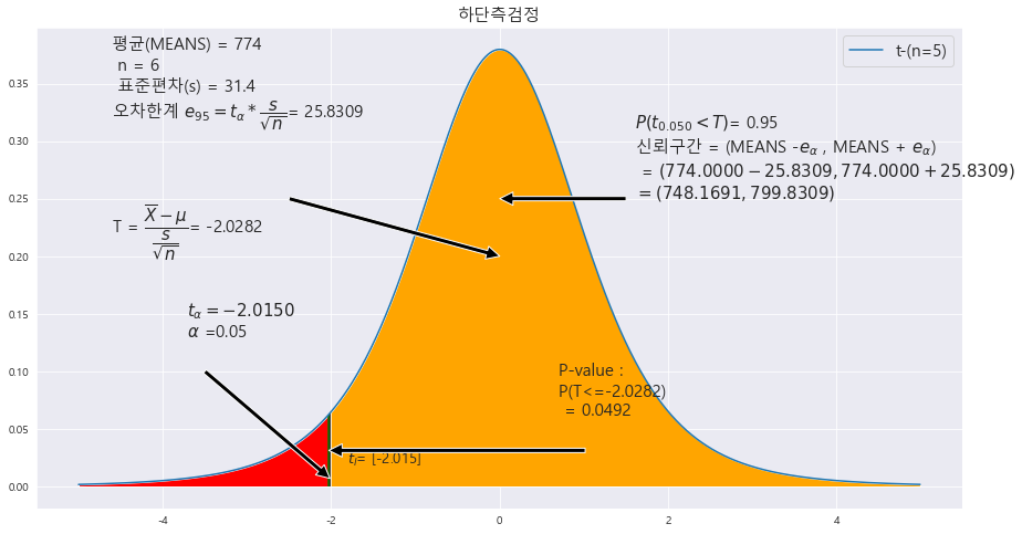
p-value : 0.0492
alpha : 0.05
p-value < alpha ==> 0.0492 < 0.05 ==> 귀무가설 H_0 : M >= 800(하단측 검정) 은 기각한다. 즉 , 유의수준 5%에서 칼슘의 섭취량이 800mg 에 부족하다.
3. t-분포에 대한 상단측검정
EX-05) 어느 대형 마트를 이용하는 고객의 지출이 1인당 평균 9만원을 초과하는지 알아보기 위하여 임의로 고객 6명을 선정하여 조사한 결과 다음과 같았다. 이마트에서 1인당 지출이 9만 원을 초과하는지 유의수준 5%에서 조사하라.
[14.8, 9.5, 11.2, 9.8, 10.2, 9.4]
H_0 : m <= 9(상단측 검정)
MEANS = 10.8167
n = 6
s = 2.0576
X = np.arange(-5,5 , .01)

fig = plt.figure(figsize=(15,8))


#
A = "14.8 9.5 11.2 9.8 10.2 9.4"
A = list(map(float, A.split(' ')))
print(A)

MEANS = round(np.mean(A) , 4)
STDS = round(np.std(A , ddof =1 ) ,4)
MO_MEAN = 9


n = len(A) #표본개수
dof_2 = [n-1] #자유도c

ax = sns.lineplot(x = X , y=scipy.stats.t(dof_2).pdf(X) )
trust = 95 #신뢰도
trust = round( (1- trust/100) , 4)
t_r =  scipy.stats.t(dof_2).ppf(1- trust)
print(t_r)
t_l = scipy.stats.t(dof_2).ppf(trust)
print(t_l)

E = round(float(t_r * STDS / math.sqrt(n)),4) #오차한계


ax.set_title('상단측검정' , fontsize = 15)
# =========================================================

ax.fill_between(X, scipy.stats.t(dof_2).pdf(X) , 0 , where = (X<=t_r)  , facecolor = 'orange') # x값 , y값 , 0 , X조건 인곳 , 색깔
area = round(float(scipy.stats.t(dof_2).cdf(t_r)),4)


plt.annotate('' , xy=(0, .2), xytext=(-2.5 , .25)  , arrowprops = dict(facecolor = 'black'))
ax.text(-4.6 , .32, f'평균(MEANS) = {MEANS}\n'  +f' n = {n} \n 표준편차(s) = {STDS}\n' +r'오차한계 $e_{%d} = t_{{\alpha}}*\dfrac{s}{\sqrt{n}}$' % ((1-  trust)*100 ) +f'= {E}' ,fontsize=15)

plt.annotate('' , xy=(0, .25), xytext=(1.5 , .25)  , arrowprops = dict(facecolor = 'black'))
ax.text(1.6 , .25, r'$P(t_{%.3f}>T)$' % (trust) + f'= {area}\n' + r'신뢰구간 = (MEANS -$e_{\alpha}$ , MEANS + $e_{\alpha}$)' +f'\n' + r' = $({%.4f} - {%.4f} , {%.4f} + {%.4f})$' % (MEANS, E , MEANS , E)  +f'\n' +r'$ = ({%.4f} , {%.4f})$' % (MEANS-E , MEANS+E)  ,fontsize=15)

# ax.vlines(x = t_r ,ymin=0 , ymax= scipy.stats.t(dof_2).pdf(t_r) , colors = 'black')
ax.vlines(x = t_r ,ymin=0 , ymax= scipy.stats.t(dof_2).pdf(t_r) , colors = 'black')


# plt.annotate('' , xy=(t_r, .007), xytext=(2.5 , .1)  , arrowprops = dict(facecolor = 'black'))
plt.annotate('' , xy=(t_r, .007), xytext=(2.5 , .1)  , arrowprops = dict(facecolor = 'black'))
# ax.text(1.71 , .13, r'$t_{\dfrac{\alpha}{2}} = {%.4f}$' % t_r + '\n' +r'$\dfrac{\alpha}{2}$ =' + f'{round(float(1- scipy.stats.t(dof_2).cdf(t_r)),3)}',fontsize=15)
ax.text(2.71 , .13, r'$t_{{\alpha}} = {%.4f}$' % t_r + '\n' +r'${\alpha}$ =' +f'{round(float(1- scipy.stats.t(dof_2).cdf(t_r)),3)}',fontsize=15)

ax.text(t_r - 1 , 0.02 , r'$t_r$' + f'= {t_r}'  , fontsize = 13)
# ax.text(t_l + .2 , 0.02 , r'$t_l$' + f'= {t_l}'  , fontsize = 13)


#==================================== 가설 검정 ==========================================


t_1 = round((MEANS - MO_MEAN)/ (STDS / math.sqrt(n)),4)

print(t_1)
t_1 = abs(t_1)
area = round(1- float(scipy.stats.t(dof_2).cdf(t_1) ),4)
ax.fill_between(X, scipy.stats.t(dof_2).pdf(X) , 0 , where =  (X>=t_1) , facecolor = 'skyblue') # x값 , y값 , 0 , X조건 인곳 , 색깔
ax.fill_between(X, scipy.stats.t(dof_2).pdf(X) , 0 , where = (X>=t_r) , facecolor = 'red') # x값 , y값 , 0 , X조건 인곳 , 색깔

ax.vlines(x= t_1, ymin= 0 , ymax= stats.t(dof_2).pdf(t_1) , color = 'green' , linestyle ='solid' , label ='{}'.format(2))
# ax.vlines(x= -t_1, ymin= 0 , ymax= stats.t(dof_2).pdf(-t_1) , color = 'green' , linestyle ='solid' , label ='{}'.format(2))

annotate_len = stats.t(dof_2).pdf(t_1) /2
plt.annotate('' , xy=(t_1, annotate_len), xytext=(-t_1/2 , annotate_len)  , arrowprops = dict(facecolor = 'black'))
# plt.annotate('' , xy=(-t_1, annotate_len), xytext=(t_1/2 , annotate_len)  , arrowprops = dict(facecolor = 'black'))
ax.text(-1.5, annotate_len+0.03 , f'P-value : \nP(T>={t_1}) \n = {area}',fontsize=15)

mo = '모평균'

ax.text(-4.6 , .22, r'T = $\dfrac{\overline{X} - {\mu}}{\dfrac{s}{\sqrt{n}}}$' + f'= { round((MEANS - MO_MEAN)/(STDS / math.sqrt(n)),4) }' ,fontsize=15)


b = ['t-(n={})'.format(i) for i in dof_2]
plt.legend(b , fontsize = 15)
p-value : 0.0415
alpha : 0.05
p-value < alpha ==> 0.0415 < 0.05 ==> 귀무가설 H_0 : m<= 9(상단측 검정) 은 기각한다. 즉 , 유의수준 5%에서 고객의 1인당 지출액이 9만원을 초과한다.
EX-06) 스마트폰에 사용되는 베터리의 수명이 하루를 초과하는지 알아보기 위하여 10개를 임의로 선정하여 조사한 결과, 평균 1.2일 , 표준편차 0.35일 이었다. 배터리의 수명이 하루를 초과하는지 유의수준 5%에서 조사하라.
H_0 : m<= 1 (상단측검정)
|X = 1.2
s = 0.35
n = 10
X = np.arange(-5,5 , .01)

fig = plt.figure(figsize=(15,8))


#
# A = "14.8 9.5 11.2 9.8 10.2 9.4"
# A = list(map(float, A.split(' ')))
# print(A)

MEANS = 1.2
STDS = 0.35
MO_MEAN = 1


n = 10 #표본개수
dof_2 = [n-1] #자유도c

ax = sns.lineplot(x = X , y=scipy.stats.t(dof_2).pdf(X) )
trust = 95 #신뢰도
trust = round( (1- trust/100) , 4)
t_r =  scipy.stats.t(dof_2).ppf(1- trust)
print(t_r)
t_l = scipy.stats.t(dof_2).ppf(trust)
print(t_l)

E = round(float(t_r * STDS / math.sqrt(n)),4) #오차한계


ax.set_title('상단측검정' , fontsize = 15)
# =========================================================

ax.fill_between(X, scipy.stats.t(dof_2).pdf(X) , 0 , where = (X<=t_r)  , facecolor = 'orange') # x값 , y값 , 0 , X조건 인곳 , 색깔
area = round(float(scipy.stats.t(dof_2).cdf(t_r)),4)


plt.annotate('' , xy=(0, .2), xytext=(-2.5 , .25)  , arrowprops = dict(facecolor = 'black'))
ax.text(-4.6 , .32, f'평균(MEANS) = {MEANS}\n'  +f' n = {n} \n 표준편차(s) = {STDS}\n' +r'오차한계 $e_{%d} = t_{{\alpha}}*\dfrac{s}{\sqrt{n}}$' % ((1-  trust)*100 ) +f'= {E}' ,fontsize=15)

plt.annotate('' , xy=(0, .25), xytext=(1.5 , .25)  , arrowprops = dict(facecolor = 'black'))
ax.text(1.6 , .25, r'$P(t_{%.3f}>T)$' % (trust) + f'= {area}\n' + r'신뢰구간 = (MEANS -$e_{\alpha}$ , MEANS + $e_{\alpha}$)' +f'\n' + r' = $({%.4f} - {%.4f} , {%.4f} + {%.4f})$' % (MEANS, E , MEANS , E)  +f'\n' +r'$ = ({%.4f} , {%.4f})$' % (MEANS-E , MEANS+E)  ,fontsize=15)

# ax.vlines(x = t_r ,ymin=0 , ymax= scipy.stats.t(dof_2).pdf(t_r) , colors = 'black')
ax.vlines(x = t_r ,ymin=0 , ymax= scipy.stats.t(dof_2).pdf(t_r) , colors = 'black')


# plt.annotate('' , xy=(t_r, .007), xytext=(2.5 , .1)  , arrowprops = dict(facecolor = 'black'))
plt.annotate('' , xy=(t_r, .007), xytext=(2.5 , .1)  , arrowprops = dict(facecolor = 'black'))
# ax.text(1.71 , .13, r'$t_{\dfrac{\alpha}{2}} = {%.4f}$' % t_r + '\n' +r'$\dfrac{\alpha}{2}$ =' + f'{round(float(1- scipy.stats.t(dof_2).cdf(t_r)),3)}',fontsize=15)
ax.text(2.71 , .13, r'$t_{{\alpha}} = {%.4f}$' % t_r + '\n' +r'${\alpha}$ =' +f'{round(float(1- scipy.stats.t(dof_2).cdf(t_r)),3)}',fontsize=15)

ax.text(t_r - 1 , 0.02 , r'$t_r$' + f'= {t_r}'  , fontsize = 13)
# ax.text(t_l + .2 , 0.02 , r'$t_l$' + f'= {t_l}'  , fontsize = 13)


#==================================== 가설 검정 ==========================================


t_1 = round((MEANS - MO_MEAN)/ (STDS / math.sqrt(n)),4)

print(t_1)
t_1 = abs(t_1)
area = round(1- float(scipy.stats.t(dof_2).cdf(t_1) ),4)
ax.fill_between(X, scipy.stats.t(dof_2).pdf(X) , 0 , where =  (X>=t_1) , facecolor = 'skyblue') # x값 , y값 , 0 , X조건 인곳 , 색깔
ax.fill_between(X, scipy.stats.t(dof_2).pdf(X) , 0 , where = (X>=t_r) , facecolor = 'red') # x값 , y값 , 0 , X조건 인곳 , 색깔

ax.vlines(x= t_1, ymin= 0 , ymax= stats.t(dof_2).pdf(t_1) , color = 'green' , linestyle ='solid' , label ='{}'.format(2))
# ax.vlines(x= -t_1, ymin= 0 , ymax= stats.t(dof_2).pdf(-t_1) , color = 'green' , linestyle ='solid' , label ='{}'.format(2))

annotate_len = stats.t(dof_2).pdf(t_1) /2
plt.annotate('' , xy=(t_1, annotate_len), xytext=(-t_1/2 , annotate_len)  , arrowprops = dict(facecolor = 'black'))
# plt.annotate('' , xy=(-t_1, annotate_len), xytext=(t_1/2 , annotate_len)  , arrowprops = dict(facecolor = 'black'))
ax.text(-1.5, annotate_len+0.03 , f'P-value : \nP(T>={t_1}) \n = {area}',fontsize=15)

mo = '모평균'

ax.text(-4.6 , .22, r'T = $\dfrac{\overline{X} - {\mu}}{\dfrac{s}{\sqrt{n}}}$' + f'= { round((MEANS - MO_MEAN)/(STDS / math.sqrt(n)),4) }' ,fontsize=15)


b = ['t-(n={})'.format(i) for i in dof_2]
plt.legend(b , fontsize = 15)
p-value : 0.0521
alpha : 0.05
p-value > alpha ==> 0.0521 > 0.05 ==> 귀무가설 H_0 : m<= 1(상단측 검정) 은 채택한다. 즉 , 배터리의 수명이 하루를 초과한다는 증거는 부족하다.
4. p-value 검정
EX-07) 어느 광역시의 보건환경연구원이 해당 광역시 주요 도로의 질소산화물은 위험수준인 0.101ppm보다 작다고 주장하였다. 이를 알아보기 위하여 이 지역의 주요 도로 18곳의 질소산화물 배출을 조사한 결과, 평균 0.098ppm , 표준편차 0.005 ppm이었다. p-value 값을 구하여 보건환경연구원의 주장에 대해 유의수준 1%에서 조사하라.
H_0 : m >= 0.101(하단측 검정)
|X = 0.098
s = 0.005
n = 18
X = np.arange(-5,5 , .01)

fig = plt.figure(figsize=(15,8))


#
# A = "1073 1067 1103 1122 1057 1096 1057 1053 1089 1102 1100 1091 1053 1138 1063 1120 1077 1091"
# A = list(map(int, A.split(' ')))


MEANS = 0.098
STDS = 0.005
MO_MEAN = 0.101


n = 18 #표본개수
dof_2 = [n-1] #자유도c

ax = sns.lineplot(x = X , y=scipy.stats.t(dof_2).pdf(X) )
trust = 99 #신뢰도
trust = round( (1- trust/100) , 4)
t_r =  scipy.stats.t(dof_2).ppf(1- trust)
print(t_r)
t_l = scipy.stats.t(dof_2).ppf(trust)
print(t_l)

E = round(float(t_r * STDS / math.sqrt(n)),4) #오차한계


ax.set_title('하단측검정' , fontsize = 15)
# =========================================================

ax.fill_between(X, scipy.stats.t(dof_2).pdf(X) , 0 , where = (X>=-t_r)  , facecolor = 'orange') # x값 , y값 , 0 , X조건 인곳 , 색깔
area = round(float(1- scipy.stats.t(dof_2).cdf(t_l)),4)


plt.annotate('' , xy=(0, .2), xytext=(-2.5 , .25)  , arrowprops = dict(facecolor = 'black'))
ax.text(-4.6 , .32, f'평균(MEANS) = {MEANS}\n'  +f' n = {n} \n 표준편차(s) = {STDS}\n' +r'오차한계 $e_{%d} = t_{{\alpha}}*\dfrac{s}{\sqrt{n}}$' % ((1-  trust)*100 ) +f'= {E}' ,fontsize=15)

plt.annotate('' , xy=(0, .25), xytext=(1.5 , .25)  , arrowprops = dict(facecolor = 'black'))
ax.text(1.6 , .25, r'$P(t_{%.3f}<T)$' % (trust) + f'= {area}\n' + r'신뢰구간 = (MEANS -$e_{\alpha}$ , MEANS + $e_{\alpha}$)' +f'\n' + r' = $({%.4f} - {%.4f} , {%.4f} + {%.4f})$' % (MEANS, E , MEANS , E)  +f'\n' +r'$ = ({%.4f} , {%.4f})$' % (MEANS-E , MEANS+E)  ,fontsize=15)

# ax.vlines(x = t_r ,ymin=0 , ymax= scipy.stats.t(dof_2).pdf(t_r) , colors = 'black')
ax.vlines(x = t_l ,ymin=0 , ymax= scipy.stats.t(dof_2).pdf(t_l) , colors = 'black')


# plt.annotate('' , xy=(t_r, .007), xytext=(2.5 , .1)  , arrowprops = dict(facecolor = 'black'))
plt.annotate('' , xy=(t_l, .007), xytext=(-3.5 , .1)  , arrowprops = dict(facecolor = 'black'))
# ax.text(1.71 , .13, r'$t_{\dfrac{\alpha}{2}} = {%.4f}$' % t_r + '\n' +r'$\dfrac{\alpha}{2}$ =' + f'{round(float(1- scipy.stats.t(dof_2).cdf(t_r)),3)}',fontsize=15)
ax.text(-3.71 , .13, r'$t_{{\alpha}} = {%.4f}$' % t_l + '\n' +r'${\alpha}$ =' +f'{round(float(scipy.stats.t(dof_2).cdf(t_l)),3)}',fontsize=15)

# ax.text(t_r - 1 , 0.02 , r'$t_r$' + f'= {t_r}'  , fontsize = 13)
ax.text(t_l + .2 , 0.02 , r'$t_l$' + f'= {t_l}'  , fontsize = 13)


#==================================== 가설 검정 ==========================================


t_1 = round((MEANS - MO_MEAN)/ (STDS / math.sqrt(n)),4)

print(t_1)
t_1 = abs(t_1)
area = round(float(scipy.stats.t(dof_2).cdf(-t_1) ),4)
ax.fill_between(X, scipy.stats.t(dof_2).pdf(X) , 0 , where =  (X<=-t_1) , facecolor = 'skyblue') # x값 , y값 , 0 , X조건 인곳 , 색깔
ax.fill_between(X, scipy.stats.t(dof_2).pdf(X) , 0 , where = (X<=t_l) , facecolor = 'red') # x값 , y값 , 0 , X조건 인곳 , 색깔

# ax.vlines(x= t_1, ymin= 0 , ymax= stats.t(dof_2).pdf(t_1) , color = 'green' , linestyle ='solid' , label ='{}'.format(2))
ax.vlines(x= -t_1, ymin= 0 , ymax= stats.t(dof_2).pdf(-t_1) , color = 'green' , linestyle ='solid' , label ='{}'.format(2))

annotate_len = stats.t(dof_2).pdf(t_1) /2
# plt.annotate('' , xy=(t_1, annotate_len), xytext=(-t_1/2 , annotate_len)  , arrowprops = dict(facecolor = 'black'))
plt.annotate('' , xy=(-t_1, annotate_len), xytext=(t_1/2 , annotate_len)  , arrowprops = dict(facecolor = 'black'))
ax.text(0.7, annotate_len+0.03 , f'P-value : \nP(T<={-t_1}) \n = {area}',fontsize=15)

mo = '모평균'

ax.text(-4.6 , .22, r'T = $\dfrac{\overline{X} - {\mu}}{\dfrac{s}{\sqrt{n}}}$' + f'= { round((MEANS - MO_MEAN)/(STDS / math.sqrt(n)),4) }' ,fontsize=15)


b = ['t-(n={})'.format(i) for i in dof_2]
plt.legend(b , fontsize = 15)
p-value : 0.0104
alpha : 0.01
p-value > alpha ==> 0.0104 > 0.01 ==> 귀무가설 H_0 : m>= 0.101(하단측 검정) 은 채택한다. 즉 , 주요도로의 위험수준은 0.101보다 크거나 같다.
EX-08) 모평균이 m<= 10이라는 주장에 대한 타당성을 조사하기 위하여 크기 25인 표본을 조사한 결과, 표본평균 10.3과 표본표준편차 2를 얻었다. p-value 값을 구하고 유의수준 5%에서 검정하라.
H_0 : m<=10 (상단측 검정)
|X = 10.3
s = 2
n = 25
X = np.arange(-5,5 , .01)

fig = plt.figure(figsize=(15,8))


#
# A = "14.8 9.5 11.2 9.8 10.2 9.4"
# A = list(map(float, A.split(' ')))
# print(A)

MEANS = 10.3
STDS = 2
MO_MEAN = 10


n = 25 #표본개수
dof_2 = [n-1] #자유도c

ax = sns.lineplot(x = X , y=scipy.stats.t(dof_2).pdf(X) )
trust = 95 #신뢰도
trust = round( (1- trust/100) , 4)
t_r =  scipy.stats.t(dof_2).ppf(1- trust)
print(t_r)
t_l = scipy.stats.t(dof_2).ppf(trust)
print(t_l)

E = round(float(t_r * STDS / math.sqrt(n)),4) #오차한계


ax.set_title('상단측검정' , fontsize = 15)
# =========================================================

ax.fill_between(X, scipy.stats.t(dof_2).pdf(X) , 0 , where = (X<=t_r)  , facecolor = 'orange') # x값 , y값 , 0 , X조건 인곳 , 색깔
area = round(float(scipy.stats.t(dof_2).cdf(t_r)),4)


plt.annotate('' , xy=(0, .2), xytext=(-2.5 , .25)  , arrowprops = dict(facecolor = 'black'))
ax.text(-4.6 , .32, f'평균(MEANS) = {MEANS}\n'  +f' n = {n} \n 표준편차(s) = {STDS}\n' +r'오차한계 $e_{%d} = t_{{\alpha}}*\dfrac{s}{\sqrt{n}}$' % ((1-  trust)*100 ) +f'= {E}' ,fontsize=15)

plt.annotate('' , xy=(0, .25), xytext=(1.5 , .25)  , arrowprops = dict(facecolor = 'black'))
ax.text(1.6 , .25, r'$P(t_{%.3f}>T)$' % (trust) + f'= {area}\n' + r'신뢰구간 = (MEANS -$e_{\alpha}$ , MEANS + $e_{\alpha}$)' +f'\n' + r' = $({%.4f} - {%.4f} , {%.4f} + {%.4f})$' % (MEANS, E , MEANS , E)  +f'\n' +r'$ = ({%.4f} , {%.4f})$' % (MEANS-E , MEANS+E)  ,fontsize=15)

# ax.vlines(x = t_r ,ymin=0 , ymax= scipy.stats.t(dof_2).pdf(t_r) , colors = 'black')
ax.vlines(x = t_r ,ymin=0 , ymax= scipy.stats.t(dof_2).pdf(t_r) , colors = 'black')


# plt.annotate('' , xy=(t_r, .007), xytext=(2.5 , .1)  , arrowprops = dict(facecolor = 'black'))
plt.annotate('' , xy=(t_r, .007), xytext=(2.5 , .1)  , arrowprops = dict(facecolor = 'black'))
# ax.text(1.71 , .13, r'$t_{\dfrac{\alpha}{2}} = {%.4f}$' % t_r + '\n' +r'$\dfrac{\alpha}{2}$ =' + f'{round(float(1- scipy.stats.t(dof_2).cdf(t_r)),3)}',fontsize=15)
ax.text(2.71 , .13, r'$t_{{\alpha}} = {%.4f}$' % t_r + '\n' +r'${\alpha}$ =' +f'{round(float(1- scipy.stats.t(dof_2).cdf(t_r)),3)}',fontsize=15)

ax.text(t_r - 1 , 0.02 , r'$t_r$' + f'= {t_r}'  , fontsize = 13)
# ax.text(t_l + .2 , 0.02 , r'$t_l$' + f'= {t_l}'  , fontsize = 13)


#==================================== 가설 검정 ==========================================


t_1 = round((MEANS - MO_MEAN)/ (STDS / math.sqrt(n)),4)

print(t_1)
t_1 = abs(t_1)
area = round(1- float(scipy.stats.t(dof_2).cdf(t_1) ),4)
ax.fill_between(X, scipy.stats.t(dof_2).pdf(X) , 0 , where =  (X>=t_1) , facecolor = 'skyblue') # x값 , y값 , 0 , X조건 인곳 , 색깔
ax.fill_between(X, scipy.stats.t(dof_2).pdf(X) , 0 , where = (X>=t_r) , facecolor = 'red') # x값 , y값 , 0 , X조건 인곳 , 색깔

ax.vlines(x= t_1, ymin= 0 , ymax= stats.t(dof_2).pdf(t_1) , color = 'green' , linestyle ='solid' , label ='{}'.format(2))
# ax.vlines(x= -t_1, ymin= 0 , ymax= stats.t(dof_2).pdf(-t_1) , color = 'green' , linestyle ='solid' , label ='{}'.format(2))

annotate_len = stats.t(dof_2).pdf(t_1) /2
plt.annotate('' , xy=(t_1, annotate_len), xytext=(-t_1/2 , annotate_len)  , arrowprops = dict(facecolor = 'black'))
# plt.annotate('' , xy=(-t_1, annotate_len), xytext=(t_1/2 , annotate_len)  , arrowprops = dict(facecolor = 'black'))
ax.text(-1.5, annotate_len+0.03 , f'P-value : \nP(T>={t_1}) \n = {area}',fontsize=15)

mo = '모평균'

ax.text(-4.6 , .22, r'T = $\dfrac{\overline{X} - {\mu}}{\dfrac{s}{\sqrt{n}}}$' + f'= { round((MEANS - MO_MEAN)/(STDS / math.sqrt(n)),4) }' ,fontsize=15)


b = ['t-(n={})'.format(i) for i in dof_2]
plt.legend(b , fontsize = 15)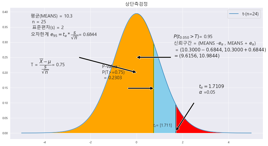
p-value : 0.2303
alpha : 0.05
p-value > alpha ==> 0.2303 > 0.01 ==> 귀무가설 H_0 : m<= 10(상단측 검정) 은 채택한다. 즉 , 모평균은 10보 다 작거나 같다.
'기초통계 > 소표본 추론' 카테고리의 다른 글
| ★카이제곱분포★모분산에 대한 소표본 추론★기초통계학-[소표본 추론-06] (0) | 2023.01.18 |
|---|---|
| ★쌍체 t-검정★기초통계학-[소표본 추론-05] (0) | 2023.01.17 |
| ★모평균의 차에 대한 소표본 가설검정★기초통계학-[소표본 추론-04] (0) | 2023.01.17 |
| ★t-분포의 합동표본분산 구하는거 기억하기★모평균 차에 대한 소표본 추정★기초통계학-[소표본 추론-03] (0) | 2023.01.17 |
| ★모평균에 대한 소표본 추론★t-분포의 신뢰구간 구하기★기초통계학-[소표본 추론-01] (0) | 2023.01.17 |