★귀무가설 설정 중요!!!!!!!(부등호가 존재)★표본평균의 차에 대한 가설 검정★모평균의 차에 대한 가설 검정★기초통계학-[연습문제 04 -12]
15. 두 모집단의 평균이 동일한지 알아보기 위하여 각각 크기 36인 표본을 조사하여 다음을 얻었다. 이것을 근거로 p-value 값을 구하고, 모평균이 동일한지 유의수준 5%에서 조사하라.
A = pd.DataFrame(columns = ['표본평균' , '모표준편차'] , index = ['A' , 'B'])
A['표본평균'] = [27.3 , 24.8]
A['모표준편차'] = [5.2 , 6.0]
A

x = np.arange(-5,5 , .001)

fig = plt.figure(figsize=(15,8))
ax = sns.lineplot(x , stats.norm.pdf(x, loc=0 , scale =1)) #정의역 범위 , 평균 = 0 , 표준편차 =1 인 정규분포 플롯

# trust = 95 #신뢰도

MEANS_A = 27.3
MEANS_B = 24.8
MEANS = round(MEANS_A-MEANS_B ,3)
std_a = 5.2
std_b = 6
n_a = 36
n_b = 36
STDS = round(math.sqrt( (std_a**2/n_a) + (std_b**2/n_b)),4)


ax.set_title('하단측검정' ,fontsize = 18)


#==========================================귀무가설 기각과 채택 ====================================================
trust = 95 #신뢰도_유의수준

t_1  = round(scipy.stats.norm.ppf((trust/100)) ,3 )
print(t_1)

ax.fill_between(x, stats.norm.pdf(x, loc=0 , scale =1) , 0 , where =  (x>=-t_1) , facecolor = 'orange') # x값 , y값 , 0 , x<=0 인곳 , 색깔
area = scipy.stats.norm.cdf(t_1)

plt.annotate('' , xy=(0, .2), xytext=(2 , .2)  , arrowprops = dict(facecolor = 'black'))
ax.text(2 , .2, r'$H_{0}$의 채택역' +f'\nP(Z>={-t_1}) : {round(area,4)}',fontsize=15)

annotate_len = stats.norm.pdf(t_1, loc=0 , scale =1) /2
# ax.vlines(x= t_1, ymin= 0 , ymax= stats.norm.pdf(t_1, loc=0 , scale =1) , color = 'green' , linestyle ='solid' , label ='{}'.format(2))
ax.vlines(x= -t_1, ymin= 0 , ymax= stats.norm.pdf(-t_1, loc=0 , scale =1) , color = 'green' , linestyle ='solid' , label ='{}'.format(2))

# ax.text(1 + t_1 , annotate_len , r'$z_{\alpha/2} = $' + f'{t_1}\n' + r'$H_{0}$의 기각역',fontsize=15)
area = 1-area
ax.text(-2.5 -t_1 , annotate_len , r'$z_{\alpha} = $' + f'{-t_1}\n' + r'$H_{0}$의 기각역'+f'\n' +r'$\alpha = {%.3f}$' % area,fontsize=15)


# plt.annotate('' , xy=(t_1, annotate_len-0.02), xytext=(t_1+ 1 , annotate_len)  , arrowprops = dict(facecolor = 'black'))
plt.annotate('' , xy=(-t_1, annotate_len), xytext=(-1-t_1 , annotate_len)  , arrowprops = dict(facecolor = 'black'))

ax.text(-5.5 , .25, f'신뢰구간 모평균에 대한 {trust}% : \n' + r'$\left( \overline{x}-\overline{y}\right)$' +f'-{t_1}' + r'$\sqrt{\dfrac{\sigma_{1}^{2}}{n}+\dfrac{\sigma_{2} ^{2}}{m}}$' +' , '+ r'$\left( \overline{x}-\overline{y}\right)$' +f'+ {t_1}' + r'$\sqrt{\dfrac{\sigma_{1}^{2}}{n}+\dfrac{\sigma_{2} ^{2}}{m}}$',fontsize=15)

ax.text(-5.5 , .2 , f'표준오차 :' + r'$\sqrt{\dfrac{\sigma_{1}^{2}}{n}+\dfrac{\sigma_{2} ^{2}}{m}}$' + f'= {round(STDS,3)}' , fontsize = 15)

ax.text(-5.5 , .15,  r'오차한계 = ${%.3f}\sqrt{\dfrac{\sigma_{1}^{2}}{n}+\dfrac{\sigma_{2} ^{2}}{m}} = $' % t_1 + f'{round(t_1 * STDS , 3)}',fontsize=15)


ax.text(2 , .35,  r'$\overline{X}_{1}$ = ' +f'{MEANS_A}'+   r' , $\overline{X}_{2}$ = ' +f'{MEANS_B}\n' + r'$\sigma_{1} = $' + f'{std_a}' + r', $\sigma_{2} = $' + f'{std_b}\n' + r'$\sqrt{n} = $' + f'{round(math.sqrt(n_a),3)}' + r', $\sqrt{m} = $' + f'{round(math.sqrt(n_b),3)}',fontsize=15)


#============================================표본평균의 정규분포화 =========================================================


z_1 = round(MEANS/ STDS ,2)
# # z_2 = round((34.5 - 35) / math.sqrt(5.5**2 / 25) , 2)
# z_1 = round(scipy.stats.norm.ppf(1 - (1-(trust/100))/2) ,3 )
z_1 = abs(z_1)
ax.fill_between(x, stats.norm.pdf(x, loc=0 , scale =1) , 0 , where = (x<=-z_1)  , facecolor = 'skyblue') # x값 , y값 , 0 , x<=0 인곳 , 색깔
ax.fill_between(x, stats.norm.pdf(x, loc=0 , scale =1) , 0 , where =  (x<=-t_1) , facecolor = 'red') # x값 , y값 , 0 , x<=0 인곳 , 색깔
area = scipy.stats.norm.cdf(-z_1)


ax.vlines(x= -z_1, ymin= 0 , ymax= stats.norm.pdf(z_1, loc=0 , scale =1) , color = 'black' , linestyle ='solid' , label ='{}'.format(2))
# ax.vlines(x= -z_1, ymin= 0 , ymax= stats.norm.pdf(-z_1, loc=0 , scale =1) , color = 'black' , linestyle ='solid' , label ='{}'.format(2))

annotate_len = stats.norm.pdf(z_1, loc=0 , scale =1) /2
# plt.annotate('' , xy=(z_1, annotate_len), xytext=(z_1+ 1 , annotate_len)  , arrowprops = dict(facecolor = 'black'))
plt.annotate('' , xy=( -z_1 ,  annotate_len), xytext=(z_1-0.05, annotate_len)  , arrowprops = dict(facecolor = 'black'))
ax.text(-.09 , annotate_len+0.01 , f'p-value \n P(Z<={-z_1})  = {round(area,4)}',fontsize=15)
# ax.text(0 , annotate_len+0.01 ,f'P(Z>={-z_1})',fontsize=15)


#
# ax.text(2 , .35,  r'$\overline{X}$ = ' +f'{MEANS}\n'+ r'$\sigma = $' + f'{STDS}\n' + r'$\sqrt{n} = $' + f'{STDS,3)}',fontsize=15)

b= 'N(0,1)'

plt.legend([b] , fontsize = 15 , loc='upper left')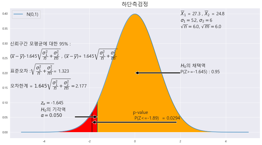
P-VALUE = 0.0294
alpha = 0.05
귀무가설 H_0 : p1 = p2 ==> ^p1 의 표본평균이 크다. ==> (하단측검정)
P-VALUE < alpha ==> 0.0294 < 0.05 ==> 귀무가설 H_0 기각 ==> 모평균이 동일하지 않다.
========================================================================================
x = np.arange(-5,5 , .001)

fig = plt.figure(figsize=(15,8))
ax = sns.lineplot(x , stats.norm.pdf(x, loc=0 , scale =1)) #정의역 범위 , 평균 = 0 , 표준편차 =1 인 정규분포 플롯

# trust = 95 #신뢰도

MEANS_A = 27.3
MEANS_B = 24.8
MEANS = round(MEANS_A-MEANS_B ,3)
std_a = 5.2
std_b = 6
n_a = 36
n_b = 36
STDS = round(math.sqrt( (std_a**2/n_a) + (std_b**2/n_b)),4)


ax.set_title('양측검정' ,fontsize = 18)


#==========================================귀무가설 기각과 채택 ====================================================
trust = 95 #신뢰도_유의수준
# trust = trust - (100-trust)
t_1  = round(scipy.stats.norm.ppf(1 - (1-(trust/100))/2) ,3 )
print(t_1)

ax.fill_between(x, stats.norm.pdf(x, loc=0 , scale =1) , 0 , where =  (x>=-t_1)  , facecolor = 'orange') # x값 , y값 , 0 , x<=0 인곳 , 색깔
area = scipy.stats.norm.cdf(t_1) - scipy.stats.norm.cdf(-t_1)

plt.annotate('' , xy=(0, .2), xytext=(2 , .2)  , arrowprops = dict(facecolor = 'black'))
ax.text(2 , .2, r'$H_{0}$의 채택역' +f'\nP({-t_1}<=Z<={t_1}) : {round(area,4)}',fontsize=15)

annotate_len = stats.norm.pdf(t_1, loc=0 , scale =1) /2
ax.vlines(x= t_1, ymin= 0 , ymax= stats.norm.pdf(t_1, loc=0 , scale =1) , color = 'green' , linestyle ='solid' , label ='{}'.format(2))
ax.vlines(x= -t_1, ymin= 0 , ymax= stats.norm.pdf(-t_1, loc=0 , scale =1) , color = 'green' , linestyle ='solid' , label ='{}'.format(2))


area = round( (1-area) / 2 , 3)
ax.text(1 + t_1 , annotate_len , r'$z_{\alpha/2} = $' + f'{t_1}\n' + r'$H_{0}$의 기각역'+f'\n' +r'$\alpha/2 = {%.3f}$' % area,fontsize=15)

ax.text(-2.5 -t_1 , annotate_len , r'$z_{\alpha/2} = $' + f'{-t_1}\n' + r'$H_{0}$의 기각역'+f'\n' +r'$\alpha/2 = {%.3f}$' % area,fontsize=15)


plt.annotate('' , xy=(t_1, annotate_len-0.02), xytext=(t_1+ 1 , annotate_len)  , arrowprops = dict(facecolor = 'black'))
plt.annotate('' , xy=(-t_1, annotate_len), xytext=(-1-t_1 , annotate_len)  , arrowprops = dict(facecolor = 'black'))


ax.text(-5.5 , .25, f'신뢰구간 모평균에 대한 {trust}% : \n' + r'$\left( \overline{x}-\overline{y}\right)$' +f'-{t_1}' + r'$\sqrt{\dfrac{\sigma_{1}^{2}}{n}+\dfrac{\sigma_{2} ^{2}}{m}}$' +' , '+ r'$\left( \overline{x}-\overline{y}\right)$' +f'+ {t_1}' + r'$\sqrt{\dfrac{\sigma_{1}^{2}}{n}+\dfrac{\sigma_{2} ^{2}}{m}}$',fontsize=15)

ax.text(-5.5 , .2 , f'표준오차 :' + r'$\sqrt{\dfrac{\sigma_{1}^{2}}{n}+\dfrac{\sigma_{2} ^{2}}{m}}$' + f'= {round(STDS,3)}' , fontsize = 15)

ax.text(-5.5 , .15,  r'오차한계 = ${%.3f}\sqrt{\dfrac{\sigma_{1}^{2}}{n}+\dfrac{\sigma_{2} ^{2}}{m}} = $' % t_1 + f'{round(t_1 * STDS , 3)}',fontsize=15)


ax.text(2 , .35,  r'$\overline{X}_{1}$ = ' +f'{MEANS_A}'+   r' , $\overline{X}_{2}$ = ' +f'{MEANS_B}\n' + r'$\sigma_{1} = $' + f'{std_a}' + r', $\sigma_{2} = $' + f'{std_b}\n' + r'$\sqrt{n} = $' + f'{round(math.sqrt(n_a),3)}' + r', $\sqrt{m} = $' + f'{round(math.sqrt(n_b),3)}',fontsize=15)


#============================================표본평균의 정규분포화 =========================================================


z_1 = round(MEANS/ STDS ,2)
# # z_2 = round((34.5 - 35) / math.sqrt(5.5**2 / 25) , 2)
# z_1 = round(scipy.stats.norm.ppf(1 - (1-(trust/100))/2) ,3 )
print(z_1)
z_1 = abs(z_1)
ax.fill_between(x, stats.norm.pdf(x, loc=0 , scale =1) , 0 , where = (x<=-z_1) | (x>=z_1)  , facecolor = 'skyblue') # x값 , y값 , 0 , x<=0 인곳 , 색깔
ax.fill_between(x, stats.norm.pdf(x, loc=0 , scale =1) , 0 , where =  (x<=-t_1) | (x>=t_1) , facecolor = 'red') # x값 , y값 , 0 , x<=0 인곳 , 색깔
area = scipy.stats.norm.cdf(-z_1) +1- scipy.stats.norm.cdf(z_1)


ax.vlines(x= z_1, ymin= 0 , ymax= stats.norm.pdf(z_1, loc=0 , scale =1) , color = 'black' , linestyle ='solid' , label ='{}'.format(2))
ax.vlines(x= -z_1, ymin= 0 , ymax= stats.norm.pdf(-z_1, loc=0 , scale =1) , color = 'black' , linestyle ='solid' , label ='{}'.format(2))

annotate_len = stats.norm.pdf(z_1, loc=0 , scale =1) /2
plt.annotate('' , xy=(z_1, annotate_len), xytext=(z_1- 1 , annotate_len)  , arrowprops = dict(facecolor = 'black'))
plt.annotate('' , xy=(-z_1, annotate_len), xytext=(1-z_1 , annotate_len)  , arrowprops = dict(facecolor = 'black'))
ax.text(-1.5 , annotate_len+0.01 , f'P-value : \nP(Z<={-z_1}) + P(Z>={z_1})  = {round(area,4)}',fontsize=15)


b= 'N(0,1)'

plt.legend([b] , fontsize = 15 , loc='upper left')

print(t_1)
==> 동일한거여서 양측 검정이 맞지 않을까?
P-VALUE = 0.0588
alpha = 0.05
귀무가설 H_0 : p1 = p2 ==>양측검정
P-VALUE > alpha ==> 0.0588 > 0.05 ==> 귀무가설 H_0 채택 ==> 모평균이 동일하다.
16. 사회계열과 공학계열 대졸 출신의 평균 임금이 동일한지 알아보기 위하여 각각 크기 50인 표본을 조사하여 다음을 얻었다. 이것을 근거로 두계열 출신의 평균 임금이 동일한지 유의수준 5%에서 조사하라.
A = pd.DataFrame(columns = ['표본평균' , '모표준편차'] , index = ['사회계열' , '공학계열'])
A['표본평균'] = [301.5 , 317.1 ]
A['모표준편차'] = [ 38.6, 43.3]
A
H_0 = 사회계열= 공학계열 (양측 검정)
x = np.arange(-5,5 , .001)

fig = plt.figure(figsize=(15,8))
ax = sns.lineplot(x , stats.norm.pdf(x, loc=0 , scale =1)) #정의역 범위 , 평균 = 0 , 표준편차 =1 인 정규분포 플롯

# trust = 95 #신뢰도

MEANS_A = 301.5
MEANS_B = 317.1
MEANS = round(MEANS_A-MEANS_B ,3)
std_a = 38.6
std_b = 43.3
n_a = 50
n_b = 50
STDS = round(math.sqrt( (std_a**2/n_a) + (std_b**2/n_b)),4)


ax.set_title('양측검정' ,fontsize = 18)


#==========================================귀무가설 기각과 채택 ====================================================
trust = 95 #신뢰도_유의수준
# trust = trust - (100-trust)
t_1  = round(scipy.stats.norm.ppf(1 - (1-(trust/100))/2) ,3 )
print(t_1)

ax.fill_between(x, stats.norm.pdf(x, loc=0 , scale =1) , 0 , where =  (x>=-t_1)  , facecolor = 'orange') # x값 , y값 , 0 , x<=0 인곳 , 색깔
area = scipy.stats.norm.cdf(t_1) - scipy.stats.norm.cdf(-t_1)

plt.annotate('' , xy=(0, .2), xytext=(2 , .2)  , arrowprops = dict(facecolor = 'black'))
ax.text(2 , .2, r'$H_{0}$의 채택역' +f'\nP({-t_1}<=Z<={t_1}) : {round(area,4)}',fontsize=15)

annotate_len = stats.norm.pdf(t_1, loc=0 , scale =1) /2
ax.vlines(x= t_1, ymin= 0 , ymax= stats.norm.pdf(t_1, loc=0 , scale =1) , color = 'green' , linestyle ='solid' , label ='{}'.format(2))
ax.vlines(x= -t_1, ymin= 0 , ymax= stats.norm.pdf(-t_1, loc=0 , scale =1) , color = 'green' , linestyle ='solid' , label ='{}'.format(2))


area = round( (1-area) / 2 , 3)
ax.text(1 + t_1 , annotate_len , r'$z_{\alpha/2} = $' + f'{t_1}\n' + r'$H_{0}$의 기각역'+f'\n' +r'$\alpha/2 = {%.3f}$' % area,fontsize=15)

ax.text(-2.5 -t_1 , annotate_len , r'$z_{\alpha/2} = $' + f'{-t_1}\n' + r'$H_{0}$의 기각역'+f'\n' +r'$\alpha/2 = {%.3f}$' % area,fontsize=15)


plt.annotate('' , xy=(t_1, annotate_len-0.02), xytext=(t_1+ 1 , annotate_len)  , arrowprops = dict(facecolor = 'black'))
plt.annotate('' , xy=(-t_1, annotate_len), xytext=(-1-t_1 , annotate_len)  , arrowprops = dict(facecolor = 'black'))


ax.text(-5.5 , .25, f'신뢰구간 모평균에 대한 {trust}% : \n' + r'$\left( \overline{x}-\overline{y}\right)$' +f'-{t_1}' + r'$\sqrt{\dfrac{\sigma_{1}^{2}}{n}+\dfrac{\sigma_{2} ^{2}}{m}}$' +' , '+ r'$\left( \overline{x}-\overline{y}\right)$' +f'+ {t_1}' + r'$\sqrt{\dfrac{\sigma_{1}^{2}}{n}+\dfrac{\sigma_{2} ^{2}}{m}}$',fontsize=15)

ax.text(-5.5 , .2 , f'표준오차 :' + r'$\sqrt{\dfrac{\sigma_{1}^{2}}{n}+\dfrac{\sigma_{2} ^{2}}{m}}$' + f'= {round(STDS,3)}' , fontsize = 15)

ax.text(-5.5 , .15,  r'오차한계 = ${%.3f}\sqrt{\dfrac{\sigma_{1}^{2}}{n}+\dfrac{\sigma_{2} ^{2}}{m}} = $' % t_1 + f'{round(t_1 * STDS , 3)}',fontsize=15)


ax.text(2 , .35,  r'$\overline{X}_{1}$ = ' +f'{MEANS_A}'+   r' , $\overline{X}_{2}$ = ' +f'{MEANS_B}\n' + r'$\sigma_{1} = $' + f'{std_a}' + r', $\sigma_{2} = $' + f'{std_b}\n' + r'$\sqrt{n} = $' + f'{round(math.sqrt(n_a),3)}' + r', $\sqrt{m} = $' + f'{round(math.sqrt(n_b),3)}',fontsize=15)


#============================================표본평균의 정규분포화 =========================================================


z_1 = round(MEANS/ STDS ,2)
# # z_2 = round((34.5 - 35) / math.sqrt(5.5**2 / 25) , 2)
# z_1 = round(scipy.stats.norm.ppf(1 - (1-(trust/100))/2) ,3 )
print(z_1)
z_1 = abs(z_1)
ax.fill_between(x, stats.norm.pdf(x, loc=0 , scale =1) , 0 , where = (x<=-z_1) | (x>=z_1)  , facecolor = 'skyblue') # x값 , y값 , 0 , x<=0 인곳 , 색깔
ax.fill_between(x, stats.norm.pdf(x, loc=0 , scale =1) , 0 , where =  (x<=-t_1) | (x>=t_1) , facecolor = 'red') # x값 , y값 , 0 , x<=0 인곳 , 색깔
area = scipy.stats.norm.cdf(-z_1) +1- scipy.stats.norm.cdf(z_1)


ax.vlines(x= z_1, ymin= 0 , ymax= stats.norm.pdf(z_1, loc=0 , scale =1) , color = 'black' , linestyle ='solid' , label ='{}'.format(2))
ax.vlines(x= -z_1, ymin= 0 , ymax= stats.norm.pdf(-z_1, loc=0 , scale =1) , color = 'black' , linestyle ='solid' , label ='{}'.format(2))

annotate_len = stats.norm.pdf(z_1, loc=0 , scale =1) /2
plt.annotate('' , xy=(z_1, annotate_len), xytext=(z_1- 1 , annotate_len)  , arrowprops = dict(facecolor = 'black'))
plt.annotate('' , xy=(-z_1, annotate_len), xytext=(1-z_1 , annotate_len)  , arrowprops = dict(facecolor = 'black'))
ax.text(-1.5 , annotate_len+0.01 , f'P-value : \nP(Z<={-z_1}) + P(Z>={z_1})  = {round(area,4)}',fontsize=15)


b= 'N(0,1)'

plt.legend([b] , fontsize = 15 , loc='upper left')

print(t_1)
귀무가설 H_0: 사회계열과 공학계열 대졸 출신의 평균 임금의 동일 여부( 사회계열 표본평균 = 공학계열 표본평균)==> 상단측 검정
p-value : 0.0574
alpha : 0.05
p-value > alpha ==> 0.0574 > 0.05 ==> 귀무가설 H_0 채택 ==> 사회계열과 공학계열 대졸 출신의 평균 임금은 동일하다.
17. 감기에 걸렸을 때 비타민 C의 효능을 알아보기 위하여, 비타민 C를 복용한 그룹과 복용하지 않은 그룹으로 나누어 회복기간을 조사하여 다음 결과를 얻었다. 이를 근거로 감기에 걸렸을 때 비타민 C가 효력이 있는지 유의수준 5%에서 조사하라.
https://knowallworld.tistory.com/307
★두 표본평균의 차에 대한 표본분포(모분산 알때 , 동일할때)★중심극한정리 활용★이표본의
1. 이표본의 표본분포 ==>지금까지는 단일 모집단의 표본에 대한 통계량의 표본분포 EX) 수능에서 남학생, 여학생 집단의 평균이 동일한지 여부 비교 ==> 비교위해서는 각각 표본을 추출하여야 한
knowallworld.tistory.com
==> 표본평균의 차에 대한 표본분포

A = pd.DataFrame(columns = ['표본평균' , '표본표준편차' , '표본의 크기'] , index = ['비타민 C를 복용한 그룹' , '비타민 C를 복용 안한 그룹'])
A['표본평균'] = [5.2 , 5.8 ]
A['표본표준편차'] = [ 1.4, 2.2]
A['표본의 크기'] = [100 , 65]
A
|X = 5.2
|Y = 5.8
귀무가설 H_0 : 비타민 C 복용 후 회복기간 >= 복용 X (하단측 검정)
대립가설 H_0 : 비타민 C 복용후 회복기간 < 복용 X
귀무가설 : 비타민 C를 복용했을 때 복용 안했을 때보다 길다.
x = np.arange(-5,5 , .001)

fig = plt.figure(figsize=(15,8))
ax = sns.lineplot(x , stats.norm.pdf(x, loc=0 , scale =1)) #정의역 범위 , 평균 = 0 , 표준편차 =1 인 정규분포 플롯

# trust = 95 #신뢰도

MEANS_A = 5.2
MEANS_B = 5.8
MEANS = round(MEANS_A-MEANS_B ,3)
std_a = 1.4
std_b = 2.2
n_a = 100
n_b = 65
STDS = round(math.sqrt( (std_a**2/n_a) + (std_b**2/n_b)),4)


ax.set_title('하단측검정' ,fontsize = 18)


#==========================================귀무가설 기각과 채택 ====================================================
trust = 95 #신뢰도_유의수준

t_1  = round(scipy.stats.norm.ppf((trust/100)) ,3 )
print(t_1)

ax.fill_between(x, stats.norm.pdf(x, loc=0 , scale =1) , 0 , where =  (x>=-t_1) , facecolor = 'orange') # x값 , y값 , 0 , x<=0 인곳 , 색깔
area = scipy.stats.norm.cdf(t_1)

plt.annotate('' , xy=(0, .2), xytext=(2 , .2)  , arrowprops = dict(facecolor = 'black'))
ax.text(2 , .2, r'$H_{0}$의 채택역' +f'\nP(Z>={-t_1}) : {round(area,4)}',fontsize=15)

annotate_len = stats.norm.pdf(t_1, loc=0 , scale =1) /2
# ax.vlines(x= t_1, ymin= 0 , ymax= stats.norm.pdf(t_1, loc=0 , scale =1) , color = 'green' , linestyle ='solid' , label ='{}'.format(2))
ax.vlines(x= -t_1, ymin= 0 , ymax= stats.norm.pdf(-t_1, loc=0 , scale =1) , color = 'green' , linestyle ='solid' , label ='{}'.format(2))

# ax.text(1 + t_1 , annotate_len , r'$z_{\alpha/2} = $' + f'{t_1}\n' + r'$H_{0}$의 기각역',fontsize=15)
area = 1-area
ax.text(-2.5 -t_1 , annotate_len , r'$z_{\alpha} = $' + f'{-t_1}\n' + r'$H_{0}$의 기각역'+f'\n' +r'$\alpha = {%.3f}$' % area,fontsize=15)


# plt.annotate('' , xy=(t_1, annotate_len-0.02), xytext=(t_1+ 1 , annotate_len)  , arrowprops = dict(facecolor = 'black'))
plt.annotate('' , xy=(-t_1, annotate_len), xytext=(-1-t_1 , annotate_len)  , arrowprops = dict(facecolor = 'black'))

ax.text(-5.5 , .25, f'신뢰구간 모평균에 대한 {trust}% : \n' + r'$\left( \overline{x}-\overline{y}\right)$' +f'-{t_1}' + r'$\sqrt{\dfrac{\sigma_{1}^{2}}{n}+\dfrac{\sigma_{2} ^{2}}{m}}$' +' , '+ r'$\left( \overline{x}-\overline{y}\right)$' +f'+ {t_1}' + r'$\sqrt{\dfrac{\sigma_{1}^{2}}{n}+\dfrac{\sigma_{2} ^{2}}{m}}$',fontsize=15)

ax.text(-5.5 , .2 , f'표준오차 :' + r'$\sqrt{\dfrac{\sigma_{1}^{2}}{n}+\dfrac{\sigma_{2} ^{2}}{m}}$' + f'= {round(STDS,3)}' , fontsize = 15)

ax.text(-5.5 , .15,  r'오차한계 = ${%.3f}\sqrt{\dfrac{\sigma_{1}^{2}}{n}+\dfrac{\sigma_{2} ^{2}}{m}} = $' % t_1 + f'{round(t_1 * STDS , 3)}',fontsize=15)


ax.text(2 , .3,  r'$\overline{X}_{1}$ = ' +f'{MEANS_A}'+   r' , $\overline{X}_{2}$ = ' +f'{MEANS_B}\n' + r'$\sigma_{1} = $' + f'{std_a}' + r', $\sigma_{2} = $' + f'{std_b}\n' + r'$\sqrt{n} = $' + f'{round(math.sqrt(n_a),3)}' + r', $\sqrt{m} = $' + f'{round(math.sqrt(n_b),3)}\n'
        + r'Z = $\dfrac{\overline{X}_{1} - \overline{X}_{2}} {\sqrt{\dfrac{\sigma_{1}^{2}}{n} + \dfrac{\sigma_{2}^{2}}{m}}}$'
        + f'= {round(MEANS / STDS,4)}' ,fontsize=15)


#============================================표본평균의 정규분포화 =========================================================


z_1 = round(MEANS/ STDS ,2)
# # z_2 = round((34.5 - 35) / math.sqrt(5.5**2 / 25) , 2)
# z_1 = round(scipy.stats.norm.ppf(1 - (1-(trust/100))/2) ,3 )
z_1 = abs(z_1)
ax.fill_between(x, stats.norm.pdf(x, loc=0 , scale =1) , 0 , where = (x<=-z_1)  , facecolor = 'skyblue') # x값 , y값 , 0 , x<=0 인곳 , 색깔
ax.fill_between(x, stats.norm.pdf(x, loc=0 , scale =1) , 0 , where =  (x<=-t_1) , facecolor = 'red') # x값 , y값 , 0 , x<=0 인곳 , 색깔
area = scipy.stats.norm.cdf(-z_1)


ax.vlines(x= -z_1, ymin= 0 , ymax= stats.norm.pdf(z_1, loc=0 , scale =1) , color = 'black' , linestyle ='solid' , label ='{}'.format(2))
# ax.vlines(x= -z_1, ymin= 0 , ymax= stats.norm.pdf(-z_1, loc=0 , scale =1) , color = 'black' , linestyle ='solid' , label ='{}'.format(2))

annotate_len = stats.norm.pdf(z_1, loc=0 , scale =1) /2
# plt.annotate('' , xy=(z_1, annotate_len), xytext=(z_1+ 1 , annotate_len)  , arrowprops = dict(facecolor = 'black'))
plt.annotate('' , xy=( -z_1 ,  annotate_len), xytext=(z_1-0.05, annotate_len)  , arrowprops = dict(facecolor = 'black'))
ax.text(-.09 , annotate_len+0.01 , f'p-value \n P(Z<={-z_1})  = {round(area,4)}',fontsize=15)
# ax.text(0 , annotate_len+0.01 ,f'P(Z>={-z_1})',fontsize=15)


#
# ax.text(2 , .35,  r'$\overline{X}$ = ' +f'{MEANS}\n'+ r'$\sigma = $' + f'{STDS}\n' + r'$\sqrt{n} = $' + f'{STDS,3)}',fontsize=15)

b= 'N(0,1)'

plt.legend([b] , fontsize = 15 , loc='upper left')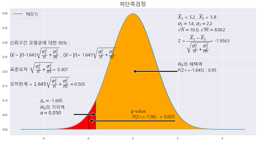
P-value = 0.0252
alpha = 0.05
귀무가설 H_0 : 비타민 C 복용 후 회복기간 >= 복용 X (하단측 검정)
p-value < alpha ==> 0.025 < 0.05 ==> 귀무가설 기각 ==> 대립가설 : 비타민 C 복용 후 회복기간 < 복용 X 후 회복기간 선정 ==> 비타민C의 복용 효과는 있다.
18. 두 그룹 A와 B의 모평균이 동일한지 알아보기 위하여 표본조사한 결과, 다음과 같았다. 이것을 근거로 모평균이 동일한지 유의수준 5%에서 조사하라.
A = pd.DataFrame(columns = ['표본평균' , '표본표준편차' , '표본의 크기'] , index = ['A' , 'B'])
A['표본평균'] = [201 , 199 ]
A['표본표준편차'] = [ 5, 6]
A['표본의 크기'] = [65 , 96]
A
H_0 : M_A = M_B(양측검정)
x = np.arange(-5,5 , .001)

fig = plt.figure(figsize=(15,8))
ax = sns.lineplot(x , stats.norm.pdf(x, loc=0 , scale =1)) #정의역 범위 , 평균 = 0 , 표준편차 =1 인 정규분포 플롯

# trust = 95 #신뢰도

MEANS_A = 201
MEANS_B = 199
MEANS = round(MEANS_A-MEANS_B ,3)
std_a = 5
std_b = 6
n_a = 65
n_b = 96
STDS = round(math.sqrt( (std_a**2/n_a) + (std_b**2/n_b)),4)


ax.set_title('양측검정' ,fontsize = 18)


#==========================================귀무가설 기각과 채택 ====================================================
trust = 95 #신뢰도_유의수준
# trust = trust - (100-trust)
t_1  = round(scipy.stats.norm.ppf(1 - (1-(trust/100))/2) ,3 )
print(t_1)

ax.fill_between(x, stats.norm.pdf(x, loc=0 , scale =1) , 0 , where =  (x>=-t_1)  , facecolor = 'orange') # x값 , y값 , 0 , x<=0 인곳 , 색깔
area = scipy.stats.norm.cdf(t_1) - scipy.stats.norm.cdf(-t_1)

plt.annotate('' , xy=(0, .2), xytext=(2 , .2)  , arrowprops = dict(facecolor = 'black'))
ax.text(2 , .2, r'$H_{0}$의 채택역' +f'\nP({-t_1}<=Z<={t_1}) : {round(area,4)}',fontsize=15)

annotate_len = stats.norm.pdf(t_1, loc=0 , scale =1) /2
ax.vlines(x= t_1, ymin= 0 , ymax= stats.norm.pdf(t_1, loc=0 , scale =1) , color = 'green' , linestyle ='solid' , label ='{}'.format(2))
ax.vlines(x= -t_1, ymin= 0 , ymax= stats.norm.pdf(-t_1, loc=0 , scale =1) , color = 'green' , linestyle ='solid' , label ='{}'.format(2))


area = round( (1-area) / 2 , 3)
ax.text(1 + t_1 , annotate_len , r'$z_{\alpha/2} = $' + f'{t_1}\n' + r'$H_{0}$의 기각역'+f'\n' +r'$\alpha/2 = {%.3f}$' % area,fontsize=15)

ax.text(-2.5 -t_1 , annotate_len , r'$z_{\alpha/2} = $' + f'{-t_1}\n' + r'$H_{0}$의 기각역'+f'\n' +r'$\alpha/2 = {%.3f}$' % area,fontsize=15)


plt.annotate('' , xy=(t_1, annotate_len-0.02), xytext=(t_1+ 1 , annotate_len)  , arrowprops = dict(facecolor = 'black'))
plt.annotate('' , xy=(-t_1, annotate_len), xytext=(-1-t_1 , annotate_len)  , arrowprops = dict(facecolor = 'black'))


ax.text(-5.5 , .25, f'신뢰구간 모평균에 대한 {trust}% : \n' + r'$\left( \overline{x}-\overline{y}\right)$' +f'-{t_1}' + r'$\sqrt{\dfrac{\sigma_{1}^{2}}{n}+\dfrac{\sigma_{2} ^{2}}{m}}$' +' , '+ r'$\left( \overline{x}-\overline{y}\right)$' +f'+ {t_1}' + r'$\sqrt{\dfrac{\sigma_{1}^{2}}{n}+\dfrac{\sigma_{2} ^{2}}{m}}$',fontsize=15)

ax.text(-5.5 , .2 , f'표준오차 :' + r'$\sqrt{\dfrac{\sigma_{1}^{2}}{n}+\dfrac{\sigma_{2} ^{2}}{m}}$' + f'= {round(STDS,3)}' , fontsize = 15)

ax.text(-5.5 , .15,  r'오차한계 = ${%.3f}\sqrt{\dfrac{\sigma_{1}^{2}}{n}+\dfrac{\sigma_{2} ^{2}}{m}} = $' % t_1 + f'{round(t_1 * STDS , 3)}',fontsize=15)


ax.text(2 , .3,  r'$\overline{X}_{1}$ = ' +f'{MEANS_A}'+   r' , $\overline{X}_{2}$ = ' +f'{MEANS_B}\n' + r'$\sigma_{1} = $' + f'{std_a}' + r', $\sigma_{2} = $' + f'{std_b}\n' + r'$\sqrt{n} = $' + f'{round(math.sqrt(n_a),3)}' + r', $\sqrt{m} = $' + f'{round(math.sqrt(n_b),3)}' + f'\n' + r'Z = $\dfrac{\overline{X}_{1} - \overline{X}_{2}} {\sqrt{\dfrac{\sigma_{1}^{2}}{n} + \dfrac{\sigma_{2}^{2}}{m}}}$'
        + f'= {round(MEANS / STDS,4)}',fontsize=15)


#============================================표본평균의 정규분포화 =========================================================


z_1 = round(MEANS/ STDS ,2)
# # z_2 = round((34.5 - 35) / math.sqrt(5.5**2 / 25) , 2)
# z_1 = round(scipy.stats.norm.ppf(1 - (1-(trust/100))/2) ,3 )
print(z_1)
z_1 = abs(z_1)
ax.fill_between(x, stats.norm.pdf(x, loc=0 , scale =1) , 0 , where = (x<=-z_1) | (x>=z_1)  , facecolor = 'skyblue') # x값 , y값 , 0 , x<=0 인곳 , 색깔
ax.fill_between(x, stats.norm.pdf(x, loc=0 , scale =1) , 0 , where =  (x<=-t_1) | (x>=t_1) , facecolor = 'red') # x값 , y값 , 0 , x<=0 인곳 , 색깔
area = scipy.stats.norm.cdf(-z_1) +1- scipy.stats.norm.cdf(z_1)


ax.vlines(x= z_1, ymin= 0 , ymax= stats.norm.pdf(z_1, loc=0 , scale =1) , color = 'black' , linestyle ='solid' , label ='{}'.format(2))
ax.vlines(x= -z_1, ymin= 0 , ymax= stats.norm.pdf(-z_1, loc=0 , scale =1) , color = 'black' , linestyle ='solid' , label ='{}'.format(2))

annotate_len = stats.norm.pdf(z_1, loc=0 , scale =1) /2
plt.annotate('' , xy=(z_1, annotate_len), xytext=(z_1- 1 , annotate_len)  , arrowprops = dict(facecolor = 'black'))
plt.annotate('' , xy=(-z_1, annotate_len), xytext=(1-z_1 , annotate_len)  , arrowprops = dict(facecolor = 'black'))
ax.text(-1.5 , annotate_len+0.01 , f'P-value : \nP(Z<={-z_1}) + P(Z>={z_1})  = {round(area,4)}',fontsize=15)


b= 'N(0,1)'

plt.legend([b] , fontsize = 15 , loc='upper left')

print(t_1)
P-value = 0.022
alpha = 0.05
귀무가설 H_0 : 모평균 A와 B가 동일여부(양측 검정)
p-value < alpha ==> 0.022 < 0.05 ==> 귀무가설 기각 ==> 모평균 A와 B는 동일하지 않다.
19. 두 회사 A와 B에서 생산된 타이어의 제동 거리가 동일한지 알아보기 위하여 두 회사 제품을 64개씩 임의로 선정하여 조사한 결과 다음과 같았다. 이것을 근거로 두 회사 타이어의 제동거리가 동일한지 유의수준 5%에서 조사하라.
A = pd.DataFrame(columns = ['평균' , '표준편차'] , index = ['A회사' , 'B회사'])
A['평균'] = [13.46 , 13.95 ]
A['표준편차'] = [1.46, 1.33]
A
|X = 13.46
|Y = 13.95
H_0 : M_A = M_B(양측 검정)
.
x = np.arange(-5,5 , .001)

fig = plt.figure(figsize=(15,8))
ax = sns.lineplot(x , stats.norm.pdf(x, loc=0 , scale =1)) #정의역 범위 , 평균 = 0 , 표준편차 =1 인 정규분포 플롯

# trust = 95 #신뢰도

MEANS_A = 13.46
MEANS_B = 13.95
MEANS = round(MEANS_A-MEANS_B ,3)
std_a = 1.46
std_b = 1.33
n_a = 64
n_b = 64
STDS = round(math.sqrt( (std_a**2/n_a) + (std_b**2/n_b)),4)


ax.set_title('양측검정' ,fontsize = 18)


#==========================================귀무가설 기각과 채택 ====================================================
trust = 95 #신뢰도_유의수준
# trust = trust - (100-trust)
t_1  = round(scipy.stats.norm.ppf(1 - (1-(trust/100))/2) ,3 )
print(t_1)

ax.fill_between(x, stats.norm.pdf(x, loc=0 , scale =1) , 0 , where =  (x>=-t_1)  , facecolor = 'orange') # x값 , y값 , 0 , x<=0 인곳 , 색깔
area = scipy.stats.norm.cdf(t_1) - scipy.stats.norm.cdf(-t_1)

plt.annotate('' , xy=(0, .2), xytext=(2 , .2)  , arrowprops = dict(facecolor = 'black'))
ax.text(2 , .2, r'$H_{0}$의 채택역' +f'\nP({-t_1}<=Z<={t_1}) : {round(area,4)}',fontsize=15)

annotate_len = stats.norm.pdf(t_1, loc=0 , scale =1) /2
ax.vlines(x= t_1, ymin= 0 , ymax= stats.norm.pdf(t_1, loc=0 , scale =1) , color = 'green' , linestyle ='solid' , label ='{}'.format(2))
ax.vlines(x= -t_1, ymin= 0 , ymax= stats.norm.pdf(-t_1, loc=0 , scale =1) , color = 'green' , linestyle ='solid' , label ='{}'.format(2))


area = round( (1-area) / 2 , 3)
ax.text(1 + t_1 , annotate_len , r'$z_{\alpha/2} = $' + f'{t_1}\n' + r'$H_{0}$의 기각역'+f'\n' +r'$\alpha/2 = {%.3f}$' % area,fontsize=15)

ax.text(-2.5 -t_1 , annotate_len , r'$z_{\alpha/2} = $' + f'{-t_1}\n' + r'$H_{0}$의 기각역'+f'\n' +r'$\alpha/2 = {%.3f}$' % area,fontsize=15)


plt.annotate('' , xy=(t_1, annotate_len-0.02), xytext=(t_1+ 1 , annotate_len)  , arrowprops = dict(facecolor = 'black'))
plt.annotate('' , xy=(-t_1, annotate_len), xytext=(-1-t_1 , annotate_len)  , arrowprops = dict(facecolor = 'black'))


ax.text(-5.5 , .25, f'신뢰구간 모평균에 대한 {trust}% : \n' + r'$\left( \overline{x}-\overline{y}\right)$' +f'-{t_1}' + r'$\sqrt{\dfrac{\sigma_{1}^{2}}{n}+\dfrac{\sigma_{2} ^{2}}{m}}$' +' , '+ r'$\left( \overline{x}-\overline{y}\right)$' +f'+ {t_1}' + r'$\sqrt{\dfrac{\sigma_{1}^{2}}{n}+\dfrac{\sigma_{2} ^{2}}{m}}$',fontsize=15)

ax.text(-5.5 , .2 , f'표준오차 :' + r'$\sqrt{\dfrac{\sigma_{1}^{2}}{n}+\dfrac{\sigma_{2} ^{2}}{m}}$' + f'= {round(STDS,3)}' , fontsize = 15)

ax.text(-5.5 , .15,  r'오차한계 = ${%.3f}\sqrt{\dfrac{\sigma_{1}^{2}}{n}+\dfrac{\sigma_{2} ^{2}}{m}} = $' % t_1 + f'{round(t_1 * STDS , 3)}',fontsize=15)


ax.text(2 , .3,  r'$\overline{X}_{1}$ = ' +f'{MEANS_A}'+   r' , $\overline{X}_{2}$ = ' +f'{MEANS_B}\n' + r'$\sigma_{1} = $' + f'{std_a}' + r', $\sigma_{2} = $' + f'{std_b}\n' + r'$\sqrt{n} = $' + f'{round(math.sqrt(n_a),3)}' + r', $\sqrt{m} = $' + f'{round(math.sqrt(n_b),3)}' + f'\n' + r'Z = $\dfrac{\overline{X}_{1} - \overline{X}_{2}} {\sqrt{\dfrac{\sigma_{1}^{2}}{n} + \dfrac{\sigma_{2}^{2}}{m}}}$'
        + f'= {round(MEANS / STDS,4)}',fontsize=15)


#============================================표본평균의 정규분포화 =========================================================


z_1 = round(MEANS/ STDS ,2)
# # z_2 = round((34.5 - 35) / math.sqrt(5.5**2 / 25) , 2)
# z_1 = round(scipy.stats.norm.ppf(1 - (1-(trust/100))/2) ,3 )
print(z_1)
z_1 = abs(z_1)
ax.fill_between(x, stats.norm.pdf(x, loc=0 , scale =1) , 0 , where = (x<=-z_1) | (x>=z_1)  , facecolor = 'skyblue') # x값 , y값 , 0 , x<=0 인곳 , 색깔
ax.fill_between(x, stats.norm.pdf(x, loc=0 , scale =1) , 0 , where =  (x<=-t_1) | (x>=t_1) , facecolor = 'red') # x값 , y값 , 0 , x<=0 인곳 , 색깔
area = scipy.stats.norm.cdf(-z_1) +1- scipy.stats.norm.cdf(z_1)


ax.vlines(x= z_1, ymin= 0 , ymax= stats.norm.pdf(z_1, loc=0 , scale =1) , color = 'black' , linestyle ='solid' , label ='{}'.format(2))
ax.vlines(x= -z_1, ymin= 0 , ymax= stats.norm.pdf(-z_1, loc=0 , scale =1) , color = 'black' , linestyle ='solid' , label ='{}'.format(2))

annotate_len = stats.norm.pdf(z_1, loc=0 , scale =1) /2
plt.annotate('' , xy=(z_1, annotate_len), xytext=(z_1- 1 , annotate_len)  , arrowprops = dict(facecolor = 'black'))
plt.annotate('' , xy=(-z_1, annotate_len), xytext=(1-z_1 , annotate_len)  , arrowprops = dict(facecolor = 'black'))
ax.text(-1.5 , annotate_len+0.01 , f'P-value : \nP(Z<={-z_1}) + P(Z>={z_1})  = {round(area,4)}',fontsize=15)


b= 'N(0,1)'

plt.legend([b] , fontsize = 15 , loc='upper left')

print(t_1)
P-value = 0.0477
alpha = 0.05
귀무가설 H_0 : 모평균 A와 B가 동일여부(양측 검정)
p-value < alpha ==> 0.0477 < 0.05 ==> 귀무가설 기각 ==> 모평균 A와 B는 동일하지 않다.
'기초통계 > 대표본 가설검정' 카테고리의 다른 글
| ★표본비율의 차에 따른 검정★합동표본비율★표본분산 모를때는 표본비율의 차로 검정★기초통계학-[연습문제 06 -14] (0) | 2023.01.16 |
|---|---|
| ★상단/하단 구분시 찾으려는 가설의 부등호 위치에 주목하자★표본평균의 차에 대한 가설 검정★기초통계학-[연습문제 05 -13] (0) | 2023.01.16 |
| ★표본비율의 정규분포화★모비율의 가설 검정★기초통계학-[연습문제 03 -11] (0) | 2023.01.16 |
| ★모평균의 가설 검정★기초통계학-[연습문제 02 -10] (1) | 2023.01.16 |
| ★=이 있는것이 귀무가설★모평균의 양측검정★모평균 <= |X 상단측 검정★모평균 >= |X 하단측검정★기초통계학-[연습문제 01 -09] (2) | 2023.01.16 |