[PYTHON - 머신러닝_캐글_실습-03]자전거 대요 수요 예측★calendar★lambda

1. 문제 : season기준이 아닌 month 기준으로 훈련 결과 값 출력

1. 데이터 전처리

import numpy as np
import pandas as pd

data_path = './bike-sharing-demand/'

train = pd.read_csv(data_path + 'train.csv') # 훈련 데이터
test = pd.read_csv(data_path + 'test.csv') # 테스트 데이터
submission = pd.read_csv(data_path + 'sampleSubmission.csv') # 제출 샘플 데이터

==> train , test , submission 데이터 불러오기

 

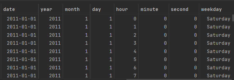
train['date'] = train['datetime'].apply(lambda x : x.split()[0]) # 날짜 피처 생성
train['datetime'] = pd.to_datetime(train['datetime'])
train['year'] = train['datetime'].dt.year # 연도

train['month'] = train['datetime'].dt.month # 월

train['day'] = train['datetime'].dt.day

train['hour'] = train['datetime'].dt.hour # 시간
train['minute'] = train['datetime'].dt.minute # 분
train['second'] = train['datetime'].dt.second # 초
train['weekday'] = train['datetime'].dt.weekday # 요일

train

import calendar
from datetime import datetime

# train['weekday'] = train['date'].apply(lambda dateString : calendar.day_name[datetime.strptime(dateString , '%Y-%m-%d').weekday()]) # weekday 출력하기(요일)


train['weekday'] = train['weekday'].apply(lambda dateString : calendar.day_name[dateString]) # weekday 출력하기(요일)
train

==> lambda 활용및 , calendar 라이브러리 활용하여 dateString의 값에 따라, 요일로 변환

dt.활용

mpl.rc('font' , size = 14) # 폰트 크기 설정
mpl.rc('axes' , titlesize = 15) # 각 축의 제목 크기 설정
figure , axes = plt.subplots(nrows=1 , ncols=2) # 3행 2열 Figure 생성
plt.tight_layout() # 그래프 사이에 여백 확보
figure.set_size_inches(10 , 9) # 전체 Figure 크기를 10x9 인치로 설정

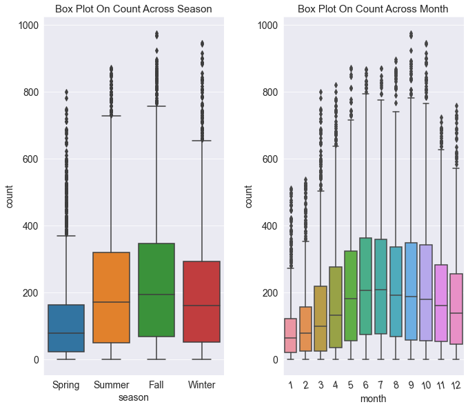
sns.boxplot(x='season' , y ='count' , data = train , ax = axes[0])
sns.boxplot(x='month' , y ='count' , data = train , ax = axes[1])
# sns.boxplot(x='workingday' , y ='count' , data = train , ax = axes[1,1])



axes[0].set(title ='Box Plot On Count Across Season')
axes[1].set(title='Box Plot On Count Across Month')
# axes[1,0].set(title='Box Plot On Count Across Holiday')
# axes[1,1].set(title='Box Plot On Count Across Workingday')

#
axes[1].tick_params(axis= 'x' , labelrotation = 10)

plt.show()

==> axes[0,1] 이 아닌 axes[0] , axes[1] 로 받는다.

month 별 예측

mpl.rc('font'  , size = 11)
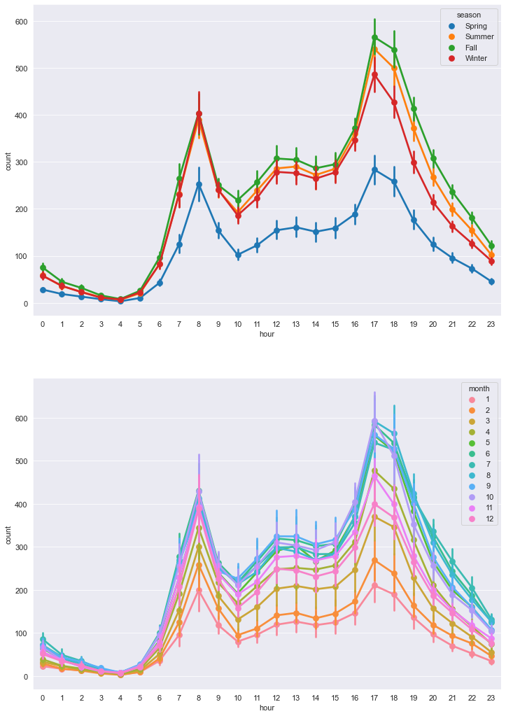
figure , axes = plt.subplots(nrows=2) # 5행 1열
figure.set_size_inches(12,18)

# STEP 2 : 서브플롯 할당
# 근무일 , 공휴일 , 요일 ,계절 , 날씨에 따른 시간대별 평균 대여 수량 포인트플롯

sns.pointplot(x='hour' , y='count' , data = train , hue='season' , ax= axes[0]) # hue로 비교하고 싶은 피처 전달
sns.pointplot(x='hour' , y='count' , data = train , hue='month' , ax= axes[1])

 

2. 모델 예측

drop_features = ['casual' , 'registered' , 'datetime' , 'date' , 'season' , 'windspeed']

all_data = all_data.drop(drop_features , axis = 1)

all_data

# 훈련 데이터의 테스트 데이터 나누기
X_train = all_data[~pd.isnull(all_data['count'])] # all_data의 count 열에서 null 이 아닌 값들에 대한 모든 열
X_test = all_data[pd.isnull(all_data['count'])] # all_data 의 count열에서 null 인 값들에 대한 모든 열

X_train

# 타깃값 count 제거
X_train = X_train.drop(['count'] , axis =1)
X_test = X_test.drop(['count'], axis =1)

y = train['count'] # 타깃값

==> 타깃값(종속변수)에 count 값 집어넣기

 

import numpy as np

def rmsle(y_true , y_pred , convertExp = True):

    if convertExp:
        y_true = np.exp(y_true)
        y_pred = np.exp(y_pred)

    # 로그변환 후 결측값을 0으로 변환
    log_true = np.nan_to_num(np.log(y_true +1))
    log_pred = np.nan_to_num(np.log(y_pred +1))


    # RMSLE 계산
    output = np.sqrt(np.mean((log_true - log_pred)**2))
    return output

==> 모델 성능 평가

 

from sklearn.linear_model import LinearRegression

linear_reg_model = LinearRegression()

log_y = np.log(y) # 타깃값 로그변환
linear_reg_model.fit(X_train , log_y) # 모델 훈련

preds = linear_reg_model.predict(X_train) # 코드 실행시 훈련된 선형 회귀 모델이 X_train 피처를 기반으로 타깃값을 예측

# 훈련시에는 훈련 데이터만, 검증시 검증 데이터만 , 테스트 시 테스트 데이터를 사용해야 한다.

# 지금처럼 훈련 시 사용한 데이터를 예측할 때 사용하는 경우는 없다.

# 시험 공부할 때 이미 풀어본 문제가 실제 시험에 나오면 안되는 이유와 같기 때문이다.

from sklearn.model_selection import GridSearchCV
from sklearn.ensemble import RandomForestRegressor
from sklearn import metrics

# 교차검증용 평가 함수(RMSLE 점수 계산)
rmsle_scorer = metrics.make_scorer(rmsle, greater_is_better= False)

# 모델 생성

randomforest_model = RandomForestRegressor()

# 그리드서치 객체 생성

rf_params = {'random_state' : [42] , 'n_estimators' : [100, 120 ,140]} # random_state는 랜덤 시드값 , n_estimators는 랜덤 포레스트를 구성하는 결정 트리 개수

gridsearch_random_forest_model = GridSearchCV(estimator= randomforest_model , param_grid= rf_params ,
                                              scoring = rmsle_scorer , cv=5)

# 그리드서치 수행

log_y = np.log(y)
gridsearch_random_forest_model.fit(X_train , log_y)

print('최적 하이퍼파라미터 : ' , gridsearch_random_forest_model.best_params_)

==> 랜덤 포레스트 모델 실행

 

==> 최적 하이퍼파라미터 :  {'n_estimators': 140, 'random_state': 42}

 

# 예측
preds = gridsearch_random_forest_model.best_estimator_.predict(X_train)

# 평가
print(f'랜덤 포레스트 회귀 RMSLE 값 : {rmsle(log_y , preds , True) : .4f}' )

==> RMSLE 값 : 0.1126

import seaborn as sns
import matplotlib.pyplot as plt

randomforest_preds = gridsearch_random_forest_model.best_estimator_.predict(X_test)

fig, ax = plt.subplots(ncols=2)
fig.set_size_inches(10,4)

sns.histplot(y, bins = 50 , ax = ax[0])
ax[0].set_title('Train Data Distribution')
sns.histplot(np.exp(randomforest_preds) , bins = 50 , ax = ax[1])
ax[1].set_title('Predicted Test Data Distribution')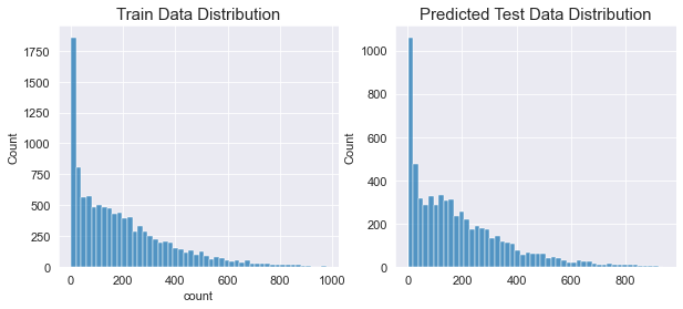

month별 예측값 량 그래프

출처 : 머신러닝·딥러닝 문제해결 전략

(Golden Rabbit , 저자 : 신백균)

※혼자 공부용