[PYTHON - 머신러닝_캐글_실습-02]자전거 대요 수요 예측★np.nan_to_num★예측과 훈련의 의미★최적 하이퍼파라미터 찾기위한 그리드 서치

1. date , year , month , hour 로 구분하기

from datetime import datetime

# 날짜 피처 생성

all_data['date'] = all_data['datetime'].apply(lambda x : x.split()[0])

all_data['year'] = all_data['datetime'].apply(lambda x : x.split()[0].split('-')[0])

all_data['month'] = all_data['datetime'].apply(lambda x : x.split()[0].split('-')[1])

all_data['hour'] = all_data['datetime'].apply(lambda x : x.split()[1].split(':')[0])

all_data['minute'] = all_data['datetime'].apply(lambda x : x.split()[1].split(':')[1])

# 요일 피처 생성

all_data['weekday'] = all_data['date'].apply(lambda dateString : datetime.strptime(dateString, '%Y-%m-%d').weekday())

# 훈련 데이터는 매달 1~19일 , 테스트 데이터는 20일~ 말일 ==> 대여 수량을 예측할 때 day 피처는 사용할 필요가 없다.

all_data['datetime'] = pd.to_datetime(all_data['datetime'])

all_data['year'] = all_data['datetime'].dt.year # 연도

all_data['month'] = all_data['datetime'].dt.month # 월

all_data['hour'] = all_data['datetime'].dt.hour # 시간

all_data['weekday'] = all_data['datetime'].dt.weekday # 요일

all_data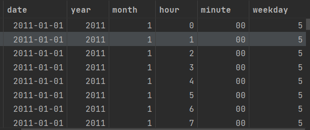

datetime 으로 생성

2. casual , registered , datetime ,date , month ,windspeed 삭제하기

drop_features = ['casual' , 'registered' , 'datetime' , 'date' , 'month' , 'windspeed']

all_data = all_data.drop(drop_features , axis = 1)

all_data

3. 데이터 나누기

# 훈련 데이터의 테스트 데이터 나누기
X_train = all_data[~pd.isnull(all_data['count'])] # all_data의 count 열에서 null 이 아닌 값들에 대한 모든 열
X_test = all_data[pd.isnull(all_data['count'])] # all_data 의 count열에서 null 인 값들에 대한 모든 열

# 타깃값 count 제거
X_train = X_train.drop(['count'] , axis =1)
X_test = X_test.drop(['count'], axis =1)

y = train['count'] # 타깃값

==> pd.isnull() 주목!!

 

4. 평가지표 계산 함수(RMSLE)

import numpy as np

def rmsle(y_true , y_pred , convertExp = True):

    if convertExp:
        y_true = np.exp(y_true)
        y_pred = np.exp(y_pred)

    # 로그변환 후 결측값을 0으로 변환
    log_true = np.nan_to_num(np.log(y_true +1))
    log_pred = np.nan_to_num(np.log(y_pred +1))


    # RMSLE 계산
    output = np.sqrt(np.mean((log_true - log_pred)**2))
    return output

==> 지수 변환하는 이유는 타깃값으로  count가 아닌 log(count)를 사용하기 때문이다. 예측한 log(count)에 지수 변환을 하면 count를 구할 수 있다.

 

==> np.nan_to_num 함수는 NaN 결측값을 모두 0으로 바꾸는 함수 이다.

 

5. 모델 훈련

1> 사이킷런의 선형 회귀모델 LinearRegression을 임포트하여 모델을 생성

from sklearn.linear_model import LinearRegression

linear_reg_model = LinearRegression()

log_y = np.log(y) # 타깃값 로그변환
linear_reg_model.fit(X_train , log_y) # 모델 훈련

==> y는 타깃값인 train['count']를 할당한 변수이다.

 

==> 선형 회귀모델을 훈련한다는 것은 독립변수(피처)인 X_train과 종속변수(타깃값) 인 log_y에 대응하는 최적의 선형 회귀 계수를 구한다는 의미이다.

 

훈련의 의미 : 

 

훈련 : 

선형회귀 훈련

==> 독립변수 x_1 , x_2 , x_3 와 종속변수 Y를 활용하여 선형 회귀계수 쉐타를 구할 수 있다.

 

==> 피처(독립변수) 와 타깃값(종속변수)이 주어졌을 때 최적의 가중치(회귀계수)를 찾는 과정

 

 

예측 : 

선형회귀 예측

==> 쉐타 값을 아는 상태에서 새로운 독립변수 x_1 , x_2 , x_3가 주어진다면 종속변수 Y를 구할 수 있다.

 

==> 최적의 가중치를 아는 상태(훈련된 모델)에서 새로운 독립변수(데이터) 가 주어졌을 때 타깃값을 추정하는 과정

 

6. 모델 성능 검증

preds = linear_reg_model.predict(X_test)

==> 훈련시에는 훈련 데이터만, 검증시 검증 데이터만 , 테스트 시 테스트 데이터를 사용해야 한다.

==>  시험 공부할 때 이미 풀어본 문제가 실제 시험에 나오면 안되는 이유와 같기 때문이다.

 

linearreg_preds =  linear_reg_model.predict(X_test) # 테스트 데이터로 예측

submission['count'] = np.exp(linearreg_preds) # 지수 변환

예측값

 

7. 성능 개선 1 : 릿지 회귀 모델

==> 릿지 회귀 모델은 L2 규제를 적용한 선형 회귀 모델이다. 규제란 모델이 훈련 데이터에 과대적합되지 않도록 해주는 방법이다.

 

==> 훈련 데이터에 과대적합되면 모델이 훈련 데이터에만 너무 잘 들어맞고, 테스트 데이터로는 제대로 예측하지 못한다.

 

 

1> 하이퍼파라미터 최적화

 

==> 그리드 서치 : 하이퍼파라미터를 격자 처럼 촘촘하게 순회하며 최적의 하이퍼파라미터 값을 찾는 기법이다.

 

==> 하이퍼파라미터를 적용한 모델마다 교차 검증하며 성능을 측정하여 성능이 가장 좋았을 때의 하이퍼파라미터 값을 찾는다.

 

from sklearn.linear_model import Ridge
from sklearn.model_selection import GridSearchCV
from sklearn import metrics

ridge_model = Ridge()

# 하이퍼파라미터 값 목록

ridge_params = {'max_iter' : [3000] , 'alpha' : [0.1 , 1, 2, 3,4, 10 ,30, 100, 200, 300 , 400 , 800, 900 , 1000]}

# 교차검증용 평가 함수(RMSLE 점수 계산)
rmsle_scorer = metrics.make_scorer(rmsle, greater_is_better= False)

# 릿지 모델은 규제를 적용한 회귀 모델이라고 한다. 릿지 모델에서 중요한 하이퍼파라미터는 alpha로 , 값이 클수록 규제 강도가 세진다.
# 적절한 규제를 적용한다면 , 즉 alpha를 적당한 크기로 하면 과대적합 문제를 개선할 수 있다.

==> alpha 값(릿지 모델의 파라미터)

 

==> 그리드 서치는 alpha값들은 순회하며 자동 테스트해준다.

gridsearch_ridge_model = GridSearchCV(estimator=ridge_model, param_grid= ridge_params, scoring= rmsle_scorer, cv=5 )# 릿지 모델 , 값 목록 , 평가 지표 , 교차 검증 분할 수 )

==>  estimator : 분류 및 회귀 모델
==>  param_grid : 딕셔너리 형태로 모델의 하이퍼파라미터명과 여러 하이퍼파라미터 값을 지정
==> scoring : 평가지표, 사이킷런에서 기본적인 평가지표를 문자열 형태로 제공.
==> 정확도는 accuracy , F1 점수는 f1 , ROC-AUC는 roc_auc , 재현율은 recall로 표시
==> make_scorer는 평가지표 계산 함수와 평가지표 점수가 높으면 좋은지 여부 등을 인수로 받는 교차 검증용 평가 함수이다.

==> cv : 교차 검증 분할 개수(기본 값은 5)

 

log_y = np.log(y) # 타깃값 로그변환
gridsearch_ridge_model.fit(X_train , log_y) # 훈련(그리드 서치)

# 코드가 일관되도록 그리드서치 객체도 모델 객체와 똑같이 fit() 메서드를 제공한다. fit()을 실행하면 객체 생성 시 param_grid에 전달된 값을 순환하면서 교차 검증으로 평가지표 점수를 계산한다. 이때 가장 좋은 성능을 보인 값을 best_params_ 속성에 저장하여 최적 값으로
# 훈련한 모델(최적 예측기)를 best_estimator_ 속성에 저장한다.

print('최적 하이퍼파라미터 : ' , gridsearch_ridge_model.best_params_)

preds = gridsearch_ridge_model.best_estimator_.predict(X_train)

# 평가

print(f'릿지 회귀 RMSLE 값 :  , {rmsle(log_y , preds , True) : .4f}')

8. 성능 개선 2 : 라쏘 회귀 모델

==> 라쏘 회귀 모델은 L1 규제를 적용한 선형 회귀 모델이다.

 

from sklearn.linear_model import Lasso

# 모델 생성

lasso_model = Lasso()

# 하이퍼파라미터 값 목록
lasso_alpha = 1/np.array([0.1 , 1 ,2 , 3, 4, 10 ,30 , 100 , 200 , 300 , 400 , 800 , 900, 1000])

lasso_params = {'max_iter' : [3000] , 'alpha' : lasso_alpha}

# 그리드서치(with 라쏘) 객체 생성
gridsearch_lasso_model = GridSearchCV(estimator= lasso_model , param_grid= lasso_params,
                                      scoring = rmsle_scorer , cv=5)

# 그리드서치 수행
log_y = np.log(y)
gridsearch_lasso_model.fit(X_train , log_y)

print('최적 하이퍼파라미터 : ', gridsearch_lasso_model.best_params_)

# 예측

preds = gridsearch_lasso_model.best_estimator_.predict(X_train)

# 평가

print(f'라쏘 회귀 RMSLE 값 : {rmsle(log_y , preds , True) : .4f}')

9. 성능 개선 3 : 랜덤 포레스트 회귀 모델

https://knowallworld.tistory.com/376

[PYTHON - 머신러닝_랜덤 포레스트]★str.split(expand= True)★K-폴드 교차검증★하이퍼파라미터 튜닝

오버피팅 : 예측 모델이 훈련 셋을 지나치게 잘 예측한다면 새로운 데이터를 예측 할 때 큰 오차를 유발 할 수 있다. ==> 훈련 셋과 테스트 셋의 예측 정확도를 줄여야 한다.

 

 

==> 랜덤으로 생성된 무수히 많은 트리를 이용하여 예측

 

==> 여러 모델을 활용하여 하나의 모델을 이루는 기법을 앙상블이라 부른다.

 

==> 앙상블 기법 : 여러 모델을 만들고 각 예측값을 투표/평균 등으로 통합하여 더 정확한 예측 도모

from sklearn.ensemble import RandomForestRegressor

# 모델 생성

randomforest_model = RandomForestRegressor()

# 그리드서치 객체 생성

rf_params = {'random_state' : [42] , 'n_estimators' : [100, 120 ,140]} 

gridsearch_random_forest_model = GridSearchCV(estimator= randomforest_model , param_grid= rf_params ,
                                              scoring = rmsle_scorer , cv=5)

# 그리드서치 수행

log_y = np.log(y)
gridsearch_random_forest_model.fit(X_train , log_y)

print('최적 하이퍼파라미터 : ' , gridsearch_random_forest_model.best_params_)

==> random_state는 랜덤 시드값 , n_estimators는 랜덤 포레스트를 구성하는 결정 트리 개수

 

10. 최종결과

import seaborn as sns
import matplotlib.pyplot as plt

randomforest_preds = gridsearch_random_forest_model.best_estimator_.predict(X_test)

fig, ax = plt.subplots(ncols=2)
fig.set_size_inches(10,4)

sns.histplot(y, bins = 50 , ax = ax[0])
ax[0].set_title('Train Data Distribution')
sns.histplot(np.exp(randomforest_preds) , bins = 50 , ax = ax[1])
ax[1].set_title('Predicted Test Data Distribution')

==> log 변환하였으므로, exp로 지수변환 해준다.

최종결과

출처 : 머신러닝·딥러닝 문제해결 전략

(Golden Rabbit , 저자 : 신백균)

※혼자 공부용