★카이제곱분포★모분산에 대한 가설검정★양측검정★상단측,하단측검정★기초통계학-[소표본 추론-07]
1. 모분산에 대한 양측검정
EX-01) 어느 지역에 거주하는 청소년이 자원봉사에 참여하는 평균시간이 하루에 4.5시간이고 표준편차는 0.3시간이라고 한다. 이것을 알아보기 위하여 이 지역의 청소년 21명을 조사한 결과, 평균 4.3시간, 표준편차 0.2시간 이었다. 유의수준 5%에서 표준편차가 0.3시간이라는 주장을 조사하라.
m = 4.5
s = 0.3
|X = 4.3
n = 21
s= 0.2
H_0 : s= 0.3(양측 검정)
X = np.arange(0,40 , .01)

fig = plt.figure(figsize=(20,12))


# A = '12.5 11.5 6.0 5.5 15.5 11.5 10.5 17.5 10.0 9.5 13.5 8.5 11.5 15.5'
# A= list(map(float , A.split(' ')))

# Vars = np.var(A , ddof=1)
Vars = 0.2**2
n = 21
dof_2 = [n-1] #자유도

trust = 95
trust = round((1- trust/100)/2,3)


STDS = math.sqrt(Vars)
MO_std = 0.3


ax = sns.lineplot(x = X , y=scipy.stats.chi2(dof_2).pdf(X) )


X_r =  scipy.stats.chi2(dof_2).ppf(1-trust)
X_l = scipy.stats.chi2(dof_2).ppf(trust)
# t_r = round( (x_0 - (0)) / (math.sqrt(33.463) * math.sqrt(1/16 + 1/16)), 3)
print(X_r)


ax.fill_between(X, scipy.stats.chi2(dof_2).pdf(X) , 0 , where = (X<=X_r) & (X>=X_l) , facecolor = 'orange')


ax.vlines(x = X_r ,ymin=0 , ymax= scipy.stats.chi2(dof_2).pdf(X_r) , colors = 'black')
ax.vlines(x = X_l ,ymin=0 , ymax= scipy.stats.chi2(dof_2).pdf(X_l) , colors = 'black')
plt.annotate('' , xy=(X_r , scipy.stats.chi2(dof_2).pdf(X_r)/2), xytext=(X_r+2 ,.01)  , arrowprops = dict(facecolor = 'black'))
plt.annotate('' , xy=(X_l , scipy.stats.chi2(dof_2).pdf(X_l)/2), xytext=(X_l - 2 , .01)  , arrowprops = dict(facecolor = 'black'))
area = 1- scipy.stats.chi2(dof_2).cdf(X_r)
ax.text(X_r , .011, r'P(X>$\chi^2_{%.3f})$' % trust + f'= {area}',fontsize=15)
ax.text(X_l- 5 , .011, r'P(X>$\chi^2_{%.3f})$' % (1-trust) + f'= {area}',fontsize=15)


ax.text(28 , 0.05 , f'n< 10에 대한 신뢰구간\n' + r'$(e_{%d})= \left(\dfrac{(n-1)s^{2}}{X^2_{\alpha/2 , n-1}} ,\dfrac{(n-1)s^{2}}{X^2_{-(\alpha/2) , n-1}} \right)$' % ((1- (trust*2))*100) + f'\n = ({round(float((n-1) * STDS**2 / X_r),5)} , {round(float((n-1) * STDS**2 / X_l),5)})' , fontsize = 16)
ax.text(28 , 0.03 ,f'n>= 10에 대한 신뢰구간\n' +  r'신뢰구간$(e_{%d}) = \left(s\sqrt{\dfrac{(n-1)}{X^2_{\alpha/2 , n-1}}} ,s\sqrt{\dfrac{(n-1)}{X^2_{-(\alpha/2) , n-1}}} \right)$' % ((1- (trust*2))*100) + f'\n = ({round(math.sqrt((n-1) * STDS**2 / X_r),4)} , {round(math.sqrt((n-1) * STDS**2 / X_l),4)})' , fontsize = 16)
ax.text(0 , 0.05 , r'카이제곱분포(V) = $\left(\dfrac{(n-1)s^{2}}{\sigma^{2}}\right)$' + f'\n n = {n}\n s = {STDS} \n ' + r'$\alpha = {%.2f}$' % (area*2) +'\n' + r'$H_0 : \sigma = {%.3f}$' % MO_std , fontsize = 16)


ax.text(X_l + 0.4 , scipy.stats.chi2(dof_2).pdf(X_l)/2 , r'$\chi^2_L= {%.4f}$' % X_l  , fontsize = 13)
ax.text(X_r - 3 , scipy.stats.chi2(dof_2).pdf(X_r)/2 , r'$\chi^2_R= {%.4f}$' % X_r   , fontsize = 13)


b = ['t-(n={})'.format(i) for i in dof_2]
plt.legend(b , fontsize = 15)


#=================================가설검정=====================================

ax.set_title('양측 검정' , fontsize = 17)

X_L_1 = (n-1) * Vars / (MO_std**2) #검정값
print(f'X_L_1 : {X_L_1}' )
X_L_1 = abs(round(X_L_1,4))

X_R_1 = round(float(scipy.stats.chi2(dof_2).ppf(1- scipy.stats.chi2(dof_2).cdf(X_L_1))),4)
print(X_R_1)
ax.fill_between(X, scipy.stats.chi2(dof_2).pdf(X) , 0 , where = (X>=X_R_1) | (X<=X_L_1) , facecolor = 'skyblue') # x값 , y값 , 0 , X조건 인곳 , 색깔
ax.fill_between(X, scipy.stats.chi2(dof_2).pdf(X) , 0 , where = (X>=X_r) | (X<=X_l) , facecolor = 'red') # x값 , y값 , 0 , X조건 인곳 , 색깔


area = round(float(scipy.stats.chi2(dof_2).cdf(X_L_1) + 1 - (scipy.stats.chi2(dof_2).cdf(X_R_1))),4)


ax.vlines(x= X_L_1, ymin= 0 , ymax= stats.chi2(dof_2).pdf(X_L_1) , color = 'green' , linestyle ='solid' , label ='{}'.format(2))
ax.vlines(x= X_R_1, ymin= 0 , ymax= stats.chi2(dof_2).pdf(X_R_1) , color = 'green' , linestyle ='solid' , label ='{}'.format(2))
#
annotate_len = stats.chi2(dof_2).pdf(X_R_1) /2
plt.annotate('' , xy=(X_L_1, annotate_len), xytext=((X_R_1-X_L_1)/2 , annotate_len)  , arrowprops = dict(facecolor = 'black'))
plt.annotate('' , xy=(X_R_1, annotate_len), xytext=((X_R_1-X_L_1)/2 , annotate_len)  , arrowprops = dict(facecolor = 'black'))
ax.text( (X_R_1-X_L_1)/2 + 5, annotate_len+0.005 , f'P-value : \nP(X<={X_L_1}) + P(X>={X_R_1}) \n = {area}',fontsize=15)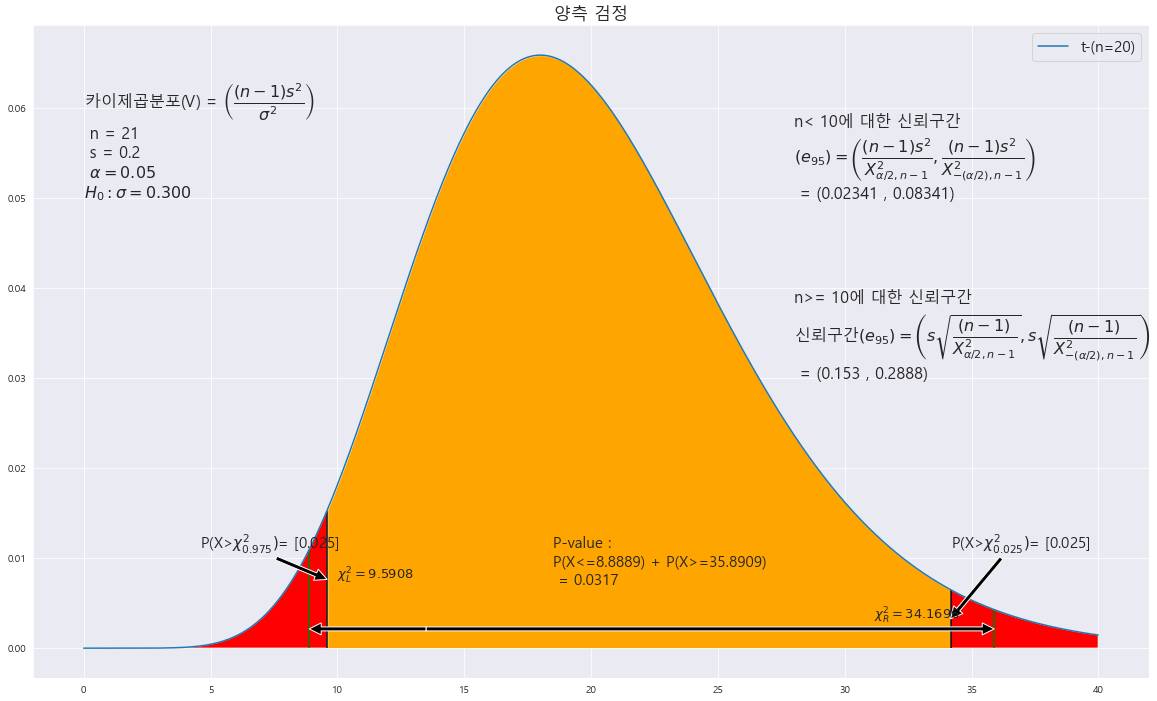
H_0 : 모표준편차 = 0.3(양측검정)
p-value : 0.0317
alpha : 0.05
p-value < alpha ==> 0.0317 < 0.05 ==> 귀무가설 H_0 : 모표준편차 = 0.3 기각한다. 즉 , 유의수준 5%에서 모표준편차는 0.3이 아니다.
EX-02) 정규모집단으로부터 크기 10인 표본을 임의로 선정하여 조사한 결과가 다음과 같았다. 모분산이 0.8이라는 주장에 대하여 유의수준 1%에서 조사하라.
X = np.arange(0,40 , .01)

fig = plt.figure(figsize=(20,12))


A = '1.5 1.1 3.6 1.5 1.7 2.1 3.2 2.5 2.8 2.9'
A= list(map(float , A.split(' ')))

Vars = np.var(A , ddof=1)
# Vars = 0.2**2
n = len(A)
dof_2 = [n-1] #자유도

trust = 99
trust = round((1- trust/100)/2,3)


STDS = math.sqrt(Vars)
MO_std = math.sqrt(0.8)


ax = sns.lineplot(x = X , y=scipy.stats.chi2(dof_2).pdf(X) )


X_r =  scipy.stats.chi2(dof_2).ppf(1-trust)
X_l = scipy.stats.chi2(dof_2).ppf(trust)
# t_r = round( (x_0 - (0)) / (math.sqrt(33.463) * math.sqrt(1/16 + 1/16)), 3)
print(f'X_r : {X_r}')
print(f'X_l : {X_l}')


ax.fill_between(X, scipy.stats.chi2(dof_2).pdf(X) , 0 , where = (X<=X_r) & (X>=X_l) , facecolor = 'orange')


ax.vlines(x = X_r ,ymin=0 , ymax= scipy.stats.chi2(dof_2).pdf(X_r) , colors = 'black')
ax.vlines(x = X_l ,ymin=0 , ymax= scipy.stats.chi2(dof_2).pdf(X_l) , colors = 'black')
plt.annotate('' , xy=(X_r , scipy.stats.chi2(dof_2).pdf(X_r)/2), xytext=(X_r+2 ,.01)  , arrowprops = dict(facecolor = 'black'))
plt.annotate('' , xy=(X_l , scipy.stats.chi2(dof_2).pdf(X_l)/2), xytext=(X_l - 2 , .01)  , arrowprops = dict(facecolor = 'black'))
area = 1- scipy.stats.chi2(dof_2).cdf(X_r)
ax.text(X_r , .011, r'P(X>$\chi^2_{%.3f})$' % trust + f'= {area}',fontsize=15)
ax.text(X_l- 5 , .011, r'P(X>$\chi^2_{%.3f})$' % (1-trust) + f'= {area}',fontsize=15)


ax.text(28 , 0.05 , f'n< 10에 대한 신뢰구간\n' + r'$(e_{%d})= \left(\dfrac{(n-1)s^{2}}{X^2_{\alpha/2 , n-1}} ,\dfrac{(n-1)s^{2}}{X^2_{-(\alpha/2) , n-1}} \right)$' % ((1- (trust*2))*100) + f'\n = ({round(float((n-1) * STDS**2 / X_r),5)} , {round(float((n-1) * STDS**2 / X_l),5)})' , fontsize = 16)
ax.text(28 , 0.03 ,f'n>= 10에 대한 신뢰구간\n' +  r'신뢰구간$(e_{%d}) = \left(s\sqrt{\dfrac{(n-1)}{X^2_{\alpha/2 , n-1}}} ,s\sqrt{\dfrac{(n-1)}{X^2_{-(\alpha/2) , n-1}}} \right)$' % ((1- (trust*2))*100) + f'\n = ({round(math.sqrt((n-1) * STDS**2 / X_r),4)} , {round(math.sqrt((n-1) * STDS**2 / X_l),4)})' , fontsize = 16)
ax.text(15 , 0.05 , r'카이제곱분포(V) = $\left(\dfrac{(n-1)s^{2}}{\sigma^{2}}\right)$' + f'\n n = {n}\n s = {STDS} \n ' + r'$\alpha = {%.2f}$' % (area*2) +'\n' + r'$H_0 : \sigma = {%.3f}$' % MO_std , fontsize = 16)


ax.text(X_l + 0.4 , scipy.stats.chi2(dof_2).pdf(X_l)/2 , r'$\chi^2_L= {%.4f}$' % X_l  , fontsize = 13)
ax.text(X_r - 3 , scipy.stats.chi2(dof_2).pdf(X_r)/2 , r'$\chi^2_R= {%.4f}$' % X_r   , fontsize = 13)


b = ['t-(n={})'.format(i) for i in dof_2]
plt.legend(b , fontsize = 15)


#=================================가설검정=====================================

ax.set_title('양측 검정' , fontsize = 17)

X_L_1 = (n-1) * Vars / (MO_std**2) #검정값
print(f'X_L_1 : {X_L_1}' )
X_L_1 = abs(round(X_L_1,4))

X_R_1 = round(float(scipy.stats.chi2(dof_2).ppf(1- scipy.stats.chi2(dof_2).cdf(X_L_1))),4)
print(f'X_R_1 : {X_R_1}' )
ax.fill_between(X, scipy.stats.chi2(dof_2).pdf(X) , 0 , where = (X>=X_R_1) | (X<=X_L_1) , facecolor = 'skyblue') # x값 , y값 , 0 , X조건 인곳 , 색깔
ax.fill_between(X, scipy.stats.chi2(dof_2).pdf(X) , 0 , where = (X>=X_r) | (X<=X_l) , facecolor = 'red') # x값 , y값 , 0 , X조건 인곳 , 색깔


area = round(float(scipy.stats.chi2(dof_2).cdf(X_L_1) + 1 - (scipy.stats.chi2(dof_2).cdf(X_R_1))),4)


ax.vlines(x= X_L_1, ymin= 0 , ymax= stats.chi2(dof_2).pdf(X_L_1) , color = 'green' , linestyle ='solid' , label ='{}'.format(2))
ax.vlines(x= X_R_1, ymin= 0 , ymax= stats.chi2(dof_2).pdf(X_R_1) , color = 'green' , linestyle ='solid' , label ='{}'.format(2))
#
annotate_len = stats.chi2(dof_2).pdf(X_R_1) /2
plt.annotate('' , xy=(X_L_1, annotate_len), xytext=((X_R_1-X_L_1)/2 , annotate_len)  , arrowprops = dict(facecolor = 'black'))
plt.annotate('' , xy=(X_R_1, annotate_len), xytext=((X_R_1-X_L_1)/2 , annotate_len)  , arrowprops = dict(facecolor = 'black'))
ax.text( (X_R_1-X_L_1)/2 + 5, annotate_len+0.005 , f'P-value : \nP(X<={X_L_1}) + P(X>={X_R_1}) \n = {area}',fontsize=15)

H_0 : 모분산 = 0.8(양측검정)
p-value : 0.8985
alpha : 0.01
p-value > alpha ==> 0.8985 > 0.01 ==> 귀무가설 H_0 : 모분산 = 0.8 채택한다. 즉 , 유의수준 1%에서 모분산은 0.8이다.
2. 모분산에 대한 하단측 검정
EX-03) 어느 단체가, 특정한 수입 자동차 연비의 표준편차가 1.2km/L 이상이라고 주장한다. 이 주장에 대해 조사하기 위하여 동일한 모델의 자동차 13대를 주행 시험한 결과 , 표준편차가 0.82km/L 였다. 자동차 연비가 정규분포를 따른다고 할 때, 이 단체의 주장을 수용할 수 잇는지 유의수준 5%에서 조사하라.
H_0 : (모표준편차)sigma >= 1.2 (하단측 검정)
n = 13
s = 0.82
X = np.arange(0,40 , .01)

fig = plt.figure(figsize=(20,12))


# A = '1.5 1.1 3.6 1.5 1.7 2.1 3.2 2.5 2.8 2.9'
# A= list(map(float , A.split(' ')))

# Vars = np.var(A , ddof=1)
Vars = 0.82**2
n = 13
dof_2 = [n-1] #자유도

trust = 95
trust = round((1- trust/100),3)


STDS = math.sqrt(Vars)
MO_std = 1.2
print(MO_std)

ax = sns.lineplot(x = X , y=scipy.stats.chi2(dof_2).pdf(X) )


# X_r =  scipy.stats.chi2(dof_2).ppf(1-trust)
X_l = scipy.stats.chi2(dof_2).ppf(trust)
# t_r = round( (x_0 - (0)) / (math.sqrt(33.463) * math.sqrt(1/16 + 1/16)), 3)
# print(f'X_r : {X_r}')
print(f'X_l : {X_l}')


ax.fill_between(X, scipy.stats.chi2(dof_2).pdf(X) , 0 , where =  (X>=X_l) , facecolor = 'orange')


# ax.vlines(x = X_r ,ymin=0 , ymax= scipy.stats.chi2(dof_2).pdf(X_r) , colors = 'black')
ax.vlines(x = X_l ,ymin=0 , ymax= scipy.stats.chi2(dof_2).pdf(X_l) , colors = 'black')
# plt.annotate('' , xy=(X_r , scipy.stats.chi2(dof_2).pdf(X_r)/2), xytext=(X_r+2 ,.01)  , arrowprops = dict(facecolor = 'black'))
plt.annotate('' , xy=(X_l , scipy.stats.chi2(dof_2).pdf(X_l)/2), xytext=(X_l - 2 , .02)  , arrowprops = dict(facecolor = 'black'))
area = scipy.stats.chi2(dof_2).cdf(X_l)
# ax.text(X_r , .011, r'P(X>$\chi^2_{%.3f})$' % trust + f'= {area}',fontsize=15)
ax.text(X_l- 5 , .021, r'P(V>$\chi^2_{%.3f})$' % (1-trust) + f'= {area}',fontsize=15)


ax.text(28 , 0.05 , f'n< 10에 대한 신뢰구간\n' + r'$(e_{%d})= \left(\dfrac{(n-1)s^{2}}{X^2_{\alpha/2 , n-1}} ,\dfrac{(n-1)s^{2}}{X^2_{-(\alpha/2) , n-1}} \right)$' % ((1- (trust*2))*100) + f'\n = ({round(float((n-1) * STDS**2 / X_r),5)} , {round(float((n-1) * STDS**2 / X_l),5)})' , fontsize = 16)
ax.text(28 , 0.03 ,f'n>= 10에 대한 신뢰구간\n' +  r'신뢰구간$(e_{%d}) = \left(s\sqrt{\dfrac{(n-1)}{X^2_{\alpha , n-1}}} ,s\sqrt{\dfrac{(n-1)}{X^2_{-(\alpha/2) , n-1}}} \right)$' % ((1- (trust))*100) + f'\n = ({round(math.sqrt((n-1) * STDS**2 / X_r),4)} , {round(math.sqrt((n-1) * STDS**2 / X_l),4)})' , fontsize = 16)
ax.text(16 , 0.05 , r'카이제곱분포(V) = $\left(\dfrac{(n-1)s^{2}}{\sigma^{2}}\right)$' + f'\n n = {n}\n s = {STDS} \n ' + r'$\alpha = {%.2f}$' % (area) +'\n' + r'$H_0 : \sigma = {%.3f}$' % MO_std , fontsize = 16)


ax.text(X_l + 0.4 , scipy.stats.chi2(dof_2).pdf(X_l)/2 , r'$\chi^2_L= {%.4f}$' % X_l  , fontsize = 13)
# ax.text(X_r - 3 , scipy.stats.chi2(dof_2).pdf(X_r)/2 , r'$\chi^2_R= {%.4f}$' % X_r   , fontsize = 13)


b = ['t-(n={})'.format(i) for i in dof_2]
plt.legend(b , fontsize = 15)


#=================================가설검정=====================================

ax.set_title('하단측 검정' , fontsize = 17)

X_L_1 = (n-1) * Vars / (MO_std**2) #검정값
print(f'X_L_1 : {X_L_1}' )
X_L_1 = abs(round(X_L_1,4))

# X_R_1 = round(float(scipy.stats.chi2(dof_2).ppf(1- scipy.stats.chi2(dof_2).cdf(X_L_1))),4)
# print(f'X_R_1 : {X_R_1}' )
ax.fill_between(X, scipy.stats.chi2(dof_2).pdf(X) , 0 , where =  (X<=X_L_1) , facecolor = 'skyblue') # x값 , y값 , 0 , X조건 인곳 , 색깔
ax.fill_between(X, scipy.stats.chi2(dof_2).pdf(X) , 0 , where =  (X<=X_l) , facecolor = 'red') # x값 , y값 , 0 , X조건 인곳 , 색깔


area = round(float(scipy.stats.chi2(dof_2).cdf(X_L_1)),4)


ax.vlines(x= X_L_1, ymin= 0 , ymax= stats.chi2(dof_2).pdf(X_L_1) , color = 'green' , linestyle ='solid' , label ='{}'.format(2))
# ax.vlines(x= X_R_1, ymin= 0 , ymax= stats.chi2(dof_2).pdf(X_R_1) , color = 'green' , linestyle ='solid' , label ='{}'.format(2))
#
annotate_len = stats.chi2(dof_2).pdf(X_R_1) /2
plt.annotate('' , xy=(X_L_1, annotate_len/2), xytext=((X_L_1)*2 , annotate_len/2)  , arrowprops = dict(facecolor = 'black'))
# plt.annotate('' , xy=(X_R_1, annotate_len), xytext=((X_R_1-X_L_1)/2 , annotate_len)  , arrowprops = dict(facecolor = 'black'))
ax.text( (X_L_1)*2 , annotate_len/2 , f'P-value : \nP(V<={X_L_1})) \n = {area}',fontsize=15)
H_0 : (모표준편차)sigma >= 1.2 (하단측 검정)
p-value : 0.0653
alpha : 0.05
p-value > alpha ==> 0.0653 > 0.05 ==> 귀무가설 H_0 : (모표준편차)sigma >= 1.2 (하단측 검정) 채택한다. 즉 , 자동차 연비의 표준편차가 1.2km/L 이상이다.
EX-04) 정규모집단에서 모표준편차가 0.09보다 작은지 알아보기 위하여, 크기 12인 표본을 추출하여 조사한 결과 표본표준편차가 0.05였다. 모표준편차가 0.09보다 작은지 유의수준 5%에서 조사하라.
H_0 : sigma(o) >= 0.09 (하단측 검정)
n = 12
s = 0.05
X = np.arange(0,40 , .01)

fig = plt.figure(figsize=(20,12))


# A = '1.5 1.1 3.6 1.5 1.7 2.1 3.2 2.5 2.8 2.9'
# A= list(map(float , A.split(' ')))

# Vars = np.var(A , ddof=1)
Vars = 0.05**2
n = 12
dof_2 = [n-1] #자유도

trust = 95
trust = round((1- trust/100),3)


STDS = math.sqrt(Vars)
MO_std = 0.09
print(MO_std)

ax = sns.lineplot(x = X , y=scipy.stats.chi2(dof_2).pdf(X) )


# X_r =  scipy.stats.chi2(dof_2).ppf(1-trust)
X_l = scipy.stats.chi2(dof_2).ppf(trust)
# t_r = round( (x_0 - (0)) / (math.sqrt(33.463) * math.sqrt(1/16 + 1/16)), 3)
# print(f'X_r : {X_r}')
print(f'X_l : {X_l}')


ax.fill_between(X, scipy.stats.chi2(dof_2).pdf(X) , 0 , where =  (X>=X_l) , facecolor = 'orange')


# ax.vlines(x = X_r ,ymin=0 , ymax= scipy.stats.chi2(dof_2).pdf(X_r) , colors = 'black')
ax.vlines(x = X_l ,ymin=0 , ymax= scipy.stats.chi2(dof_2).pdf(X_l) , colors = 'black')
# plt.annotate('' , xy=(X_r , scipy.stats.chi2(dof_2).pdf(X_r)/2), xytext=(X_r+2 ,.01)  , arrowprops = dict(facecolor = 'black'))
plt.annotate('' , xy=(X_l , scipy.stats.chi2(dof_2).pdf(X_l)/2), xytext=(X_l - 2 , .02)  , arrowprops = dict(facecolor = 'black'))
area = scipy.stats.chi2(dof_2).cdf(X_l)
# ax.text(X_r , .011, r'P(X>$\chi^2_{%.3f})$' % trust + f'= {area}',fontsize=15)
ax.text(X_l- 5 , .021, r'P(V>$\chi^2_{%.3f})$' % (1-trust) + f'= {area}',fontsize=15)


ax.text(28 , 0.05 , f'n< 10에 대한 신뢰구간\n' + r'$(e_{%d})= \left(\dfrac{(n-1)s^{2}}{X^2_{\alpha/2 , n-1}} ,\dfrac{(n-1)s^{2}}{X^2_{-(\alpha/2) , n-1}} \right)$' % ((1- (trust*2))*100) + f'\n = ({round(float((n-1) * STDS**2 / X_r),5)} , {round(float((n-1) * STDS**2 / X_l),5)})' , fontsize = 16)
ax.text(28 , 0.03 ,f'n>= 10에 대한 신뢰구간\n' +  r'신뢰구간$(e_{%d}) = \left(s\sqrt{\dfrac{(n-1)}{X^2_{\alpha , n-1}}} ,s\sqrt{\dfrac{(n-1)}{X^2_{-(\alpha/2) , n-1}}} \right)$' % ((1- (trust))*100) + f'\n = ({round(math.sqrt((n-1) * STDS**2 / X_r),4)} , {round(math.sqrt((n-1) * STDS**2 / X_l),4)})' , fontsize = 16)
ax.text(16 , 0.05 , r'카이제곱분포(V) = $\left(\dfrac{(n-1)s^{2}}{\sigma^{2}}\right)$' + f'\n n = {n}\n s = {STDS} \n ' + r'$\alpha = {%.2f}$' % (area) +'\n' + r'$H_0 : \sigma = {%.3f}$' % MO_std , fontsize = 16)


ax.text(X_l + 0.4 , scipy.stats.chi2(dof_2).pdf(X_l)/2 , r'$\chi^2_L= {%.4f}$' % X_l  , fontsize = 13)
# ax.text(X_r - 3 , scipy.stats.chi2(dof_2).pdf(X_r)/2 , r'$\chi^2_R= {%.4f}$' % X_r   , fontsize = 13)


b = ['t-(n={})'.format(i) for i in dof_2]
plt.legend(b , fontsize = 15)


#=================================가설검정=====================================

ax.set_title('하단측 검정' , fontsize = 17)

X_L_1 = (n-1) * Vars / (MO_std**2) #검정값
print(f'X_L_1 : {X_L_1}' )
X_L_1 = abs(round(X_L_1,4))

# X_R_1 = round(float(scipy.stats.chi2(dof_2).ppf(1- scipy.stats.chi2(dof_2).cdf(X_L_1))),4)
# print(f'X_R_1 : {X_R_1}' )
ax.fill_between(X, scipy.stats.chi2(dof_2).pdf(X) , 0 , where =  (X<=X_L_1) , facecolor = 'skyblue') # x값 , y값 , 0 , X조건 인곳 , 색깔
ax.fill_between(X, scipy.stats.chi2(dof_2).pdf(X) , 0 , where =  (X<=X_l) , facecolor = 'red') # x값 , y값 , 0 , X조건 인곳 , 색깔


area = round(float(scipy.stats.chi2(dof_2).cdf(X_L_1)),4)


ax.vlines(x= X_L_1, ymin= 0 , ymax= stats.chi2(dof_2).pdf(X_L_1) , color = 'green' , linestyle ='solid' , label ='{}'.format(2))
# ax.vlines(x= X_R_1, ymin= 0 , ymax= stats.chi2(dof_2).pdf(X_R_1) , color = 'green' , linestyle ='solid' , label ='{}'.format(2))
#
annotate_len = stats.chi2(dof_2).pdf(X_L_1) /2
plt.annotate('' , xy=(X_L_1, annotate_len/2), xytext=((X_L_1)*2 , annotate_len/2)  , arrowprops = dict(facecolor = 'black'))
# plt.annotate('' , xy=(X_R_1, annotate_len), xytext=((X_R_1-X_L_1)/2 , annotate_len)  , arrowprops = dict(facecolor = 'black'))
ax.text( (X_L_1)*2 , annotate_len/2 , f'P-value : \nP(V<={X_L_1})) \n = {area}',fontsize=15)

H_0 : (모표준편차)sigma >= 0.09 (하단측 검정)
p-value : 0.0156
alpha : 0.05
p-value < alpha ==> 0.0156 < 0.05 ==> 귀무가설 H_0 : (모표준편차)sigma >= 0.09 (하단측 검정) 기각한다. 즉 , 모표준편차가 0.09보다 작다.
3. 모분산에 대한 상단측 검정
EX-05) 어느 생수 회사에서 자신들이 생산하는 생수 페트병의 순수 용량은 평균 1.5L , 분산은 0.3L 이하라고 주장한다. 이것을 확인하기 위하여 임의로 페트병 15개를 수거하여 측정한 결과 , 분산이 0.48L였다. 이 생수 회사의 주장이 타당한지 유의수준 5%에서 조사하라.
H_0 : 모분산 <= 0.3 (상단측검정)
n = 15
s**2 = 0.48
X = np.arange(0,40 , .01)

fig = plt.figure(figsize=(20,12))


# A = '1.5 1.1 3.6 1.5 1.7 2.1 3.2 2.5 2.8 2.9'
# A= list(map(float , A.split(' ')))

Vars = 0.48
# Vars = 0.2**2
n = 15
dof_2 = [n-1] #자유도

trust = 95
trust = round((1- trust/100),3)


STDS = math.sqrt(Vars)
MO_std = math.sqrt(0.3)
print(MO_std)

ax = sns.lineplot(x = X , y=scipy.stats.chi2(dof_2).pdf(X) )


X_r =  scipy.stats.chi2(dof_2).ppf(1-trust)
X_l = scipy.stats.chi2(dof_2).ppf(trust)
# t_r = round( (x_0 - (0)) / (math.sqrt(33.463) * math.sqrt(1/16 + 1/16)), 3)
print(f'X_r : {X_r}')
print(f'X_l : {X_l}')


ax.fill_between(X, scipy.stats.chi2(dof_2).pdf(X) , 0 , where = (X<=X_r) , facecolor = 'orange')


ax.vlines(x = X_r ,ymin=0 , ymax= scipy.stats.chi2(dof_2).pdf(X_r) , colors = 'black')
# ax.vlines(x = X_l ,ymin=0 , ymax= scipy.stats.chi2(dof_2).pdf(X_l) , colors = 'black')
plt.annotate('' , xy=(X_r , scipy.stats.chi2(dof_2).pdf(X_r)/2), xytext=(X_r+2 ,.01)  , arrowprops = dict(facecolor = 'black'))
# plt.annotate('' , xy=(X_l , scipy.stats.chi2(dof_2).pdf(X_l)/2), xytext=(X_l - 2 , .01)  , arrowprops = dict(facecolor = 'black'))
area = 1- scipy.stats.chi2(dof_2).cdf(X_r)
ax.text(X_r , .011, r'P(X>$\chi^2_{%.3f})$' % trust + f'= {area}',fontsize=15)
# ax.text(X_l- 5 , .011, r'P(X>$\chi^2_{%.3f})$' % (1-trust) + f'= {area}',fontsize=15)


ax.text(28 , 0.05 , f'n< 10에 대한 신뢰구간\n' + r'$(e_{%d})= \left(\dfrac{(n-1)s^{2}}{X^2_{\alpha/2 , n-1}} ,\dfrac{(n-1)s^{2}}{X^2_{-(\alpha/2) , n-1}} \right)$' % ((1- (trust*2))*100) + f'\n = ({round(float((n-1) * STDS**2 / X_r),5)} , {round(float((n-1) * STDS**2 / X_l),5)})' , fontsize = 16)
ax.text(28 , 0.03 ,f'n>= 10에 대한 신뢰구간\n' +  r'신뢰구간$(e_{%d}) = \left(s\sqrt{\dfrac{(n-1)}{X^2_{\alpha , n-1}}} ,s\sqrt{\dfrac{(n-1)}{X^2_{-(\alpha/2) , n-1}}} \right)$' % ((1- (trust))*100) + f'\n = ({round(math.sqrt((n-1) * STDS**2 / X_r),4)} , {round(math.sqrt((n-1) * STDS**2 / X_l),4)})' , fontsize = 16)
ax.text(15 , 0.05 , r'카이제곱분포(V) = $\left(\dfrac{(n-1)s^{2}}{\sigma^{2}}\right)$' + f'\n n = {n}\n s = {STDS} \n ' + r'$\alpha = {%.2f}$' % (area) +'\n' + r'$H_0 : \sigma^2 <= {%.3f}$' % (MO_std**2) , fontsize = 16)


# ax.text(X_l + 0.4 , scipy.stats.chi2(dof_2).pdf(X_l)/2 , r'$\chi^2_L= {%.4f}$' % X_l  , fontsize = 13)
ax.text(X_r - 3 , scipy.stats.chi2(dof_2).pdf(X_r)/2 , r'$\chi^2_R= {%.4f}$' % X_r   , fontsize = 13)


b = ['t-(n={})'.format(i) for i in dof_2]
plt.legend(b , fontsize = 15)


#=================================가설검정=====================================

ax.set_title('상단측 검정' , fontsize = 17)

X_R_1 = (n-1) * Vars / (MO_std**2) #검정값
print(f'X_R_1 : {X_R_1}' )
X_R_1 = abs(round(X_R_1,4))
#
# X_R_1 = round(float(scipy.stats.chi2(dof_2).ppf(1- scipy.stats.chi2(dof_2).cdf(X_L_1))),4)
# print(f'X_R_1 : {X_R_1}' )
ax.fill_between(X, scipy.stats.chi2(dof_2).pdf(X) , 0 , where = (X>=X_R_1) , facecolor = 'skyblue') # x값 , y값 , 0 , X조건 인곳 , 색깔
ax.fill_between(X, scipy.stats.chi2(dof_2).pdf(X) , 0 , where = (X>=X_r) , facecolor = 'red') # x값 , y값 , 0 , X조건 인곳 , 색깔


area = round(float( 1 - (scipy.stats.chi2(dof_2).cdf(X_R_1))),4)


# ax.vlines(x= X_L_1, ymin= 0 , ymax= stats.chi2(dof_2).pdf(X_L_1) , color = 'green' , linestyle ='solid' , label ='{}'.format(2))
ax.vlines(x= X_R_1, ymin= 0 , ymax= stats.chi2(dof_2).pdf(X_R_1) , color = 'green' , linestyle ='solid' , label ='{}'.format(2))
#
annotate_len = stats.chi2(dof_2).pdf(X_R_1) /2
# plt.annotate('' , xy=(X_L_1, annotate_len), xytext=((X_R_1-X_L_1)/2 , annotate_len)  , arrowprops = dict(facecolor = 'black'))
plt.annotate('' , xy=(X_R_1, annotate_len), xytext=((X_R_1)/2 , annotate_len)  , arrowprops = dict(facecolor = 'black'))
ax.text( (X_R_1)/2 + 5, annotate_len+0.005 , f'P-value : \n P(X>={X_R_1}) \n = {area}',fontsize=15)
H_0 : (모분산)sigma^2 <= 0.548 (상단측 검정)
p-value : 0.0708
alpha : 0.05
p-value > alpha ==> 0.0708 > 0.05 ==> 귀무가설 H_0 : (모분산)sigma^2 <= 0.3 (상단측 검정) 채택한다. 즉 , 모분산이 0.3보다 작다.
EX-06) 정규모집단에서 크기 17인 표본을 조사하여 표본평균 15.1과 표준편차 2.7을 얻었다. 가설 H_0: 모분산<=4.5를 유의수준 5%에서 조사하라.
H_0 : 모분산 <= 4.5(상단측 검정)
n = 17
|x = 15.1
s = 2.7
X = np.arange(0,40 , .01)

fig = plt.figure(figsize=(20,12))


# A = '1.5 1.1 3.6 1.5 1.7 2.1 3.2 2.5 2.8 2.9'
# A= list(map(float , A.split(' ')))

Vars = 2.7**2
# Vars = 0.2**2
n = 17
dof_2 = [n-1] #자유도

trust = 95
trust = round((1- trust/100),3)


STDS = math.sqrt(Vars)
MO_std = math.sqrt(4.5)
print(MO_std)

ax = sns.lineplot(x = X , y=scipy.stats.chi2(dof_2).pdf(X) )


X_r =  scipy.stats.chi2(dof_2).ppf(1-trust)
X_l = scipy.stats.chi2(dof_2).ppf(trust)
# t_r = round( (x_0 - (0)) / (math.sqrt(33.463) * math.sqrt(1/16 + 1/16)), 3)
print(f'X_r : {X_r}')
print(f'X_l : {X_l}')


ax.fill_between(X, scipy.stats.chi2(dof_2).pdf(X) , 0 , where = (X<=X_r) , facecolor = 'orange')


ax.vlines(x = X_r ,ymin=0 , ymax= scipy.stats.chi2(dof_2).pdf(X_r) , colors = 'black')
# ax.vlines(x = X_l ,ymin=0 , ymax= scipy.stats.chi2(dof_2).pdf(X_l) , colors = 'black')
plt.annotate('' , xy=(X_r , scipy.stats.chi2(dof_2).pdf(X_r)/2), xytext=(X_r+2 ,.01)  , arrowprops = dict(facecolor = 'black'))
# plt.annotate('' , xy=(X_l , scipy.stats.chi2(dof_2).pdf(X_l)/2), xytext=(X_l - 2 , .01)  , arrowprops = dict(facecolor = 'black'))
area = 1- scipy.stats.chi2(dof_2).cdf(X_r)
ax.text(X_r , .011, r'P(X>$\chi^2_{%.3f})$' % trust + f'= {area}',fontsize=15)
# ax.text(X_l- 5 , .011, r'P(X>$\chi^2_{%.3f})$' % (1-trust) + f'= {area}',fontsize=15)


ax.text(28 , 0.05 , f'n< 10에 대한 신뢰구간\n' + r'$(e_{%d})= \left(\dfrac{(n-1)s^{2}}{X^2_{\alpha/2 , n-1}} ,\dfrac{(n-1)s^{2}}{X^2_{-(\alpha/2) , n-1}} \right)$' % ((1- (trust*2))*100) + f'\n = ({round(float((n-1) * STDS**2 / X_r),5)} , {round(float((n-1) * STDS**2 / X_l),5)})' , fontsize = 16)
ax.text(28 , 0.03 ,f'n>= 10에 대한 신뢰구간\n' +  r'신뢰구간$(e_{%d}) = \left(s\sqrt{\dfrac{(n-1)}{X^2_{\alpha , n-1}}} ,s\sqrt{\dfrac{(n-1)}{X^2_{-(\alpha/2) , n-1}}} \right)$' % ((1- (trust))*100) + f'\n = ({round(math.sqrt((n-1) * STDS**2 / X_r),4)} , {round(math.sqrt((n-1) * STDS**2 / X_l),4)})' , fontsize = 16)
ax.text(15 , 0.05 , r'카이제곱분포(V) = $\left(\dfrac{(n-1)s^{2}}{\sigma^{2}}\right)$' + f'\n n = {n}\n s = {STDS} \n ' + r'$\alpha = {%.2f}$' % (area) +'\n' + r'$H_0 : \sigma^2 <= {%.3f}$' % (MO_std**2) , fontsize = 16)


# ax.text(X_l + 0.4 , scipy.stats.chi2(dof_2).pdf(X_l)/2 , r'$\chi^2_L= {%.4f}$' % X_l  , fontsize = 13)
ax.text(X_r - 3 , scipy.stats.chi2(dof_2).pdf(X_r)/4 , r'$\chi^2_R= {%.4f}$' % X_r   , fontsize = 13)


b = ['t-(n={})'.format(i) for i in dof_2]
plt.legend(b , fontsize = 15)


#=================================가설검정=====================================

ax.set_title('상단측 검정' , fontsize = 17)

X_R_1 = (n-1) * Vars / (MO_std**2) #검정값
print(f'X_R_1 : {X_R_1}' )
X_R_1 = abs(round(X_R_1,4))
#
# X_R_1 = round(float(scipy.stats.chi2(dof_2).ppf(1- scipy.stats.chi2(dof_2).cdf(X_L_1))),4)
# print(f'X_R_1 : {X_R_1}' )
ax.fill_between(X, scipy.stats.chi2(dof_2).pdf(X) , 0 , where = (X>=X_R_1) , facecolor = 'skyblue') # x값 , y값 , 0 , X조건 인곳 , 색깔
ax.fill_between(X, scipy.stats.chi2(dof_2).pdf(X) , 0 , where = (X>=X_r) , facecolor = 'red') # x값 , y값 , 0 , X조건 인곳 , 색깔


area = round(float( 1 - (scipy.stats.chi2(dof_2).cdf(X_R_1))),4)


# ax.vlines(x= X_L_1, ymin= 0 , ymax= stats.chi2(dof_2).pdf(X_L_1) , color = 'green' , linestyle ='solid' , label ='{}'.format(2))
ax.vlines(x= X_R_1, ymin= 0 , ymax= stats.chi2(dof_2).pdf(X_R_1) , color = 'green' , linestyle ='solid' , label ='{}'.format(2))
#
annotate_len = stats.chi2(dof_2).pdf(X_R_1) /2
# plt.annotate('' , xy=(X_L_1, annotate_len), xytext=((X_R_1-X_L_1)/2 , annotate_len)  , arrowprops = dict(facecolor = 'black'))
plt.annotate('' , xy=(X_R_1, annotate_len), xytext=((X_R_1)/2 , annotate_len)  , arrowprops = dict(facecolor = 'black'))
ax.text( (X_R_1)/2 + 5, annotate_len+0.005 , f'P-value : \n P(X>={X_R_1}) \n = {area}',fontsize=15)

H_0 : (모분산)sigma^2 <= 4.5 (상단측 검정)
p-value : 0.0552
alpha : 0.05
p-value > alpha ==> 0.0552 > 0.05 ==> 귀무가설 H_0 : (모분산)sigma^2 <= 4.5 (상단측 검정) 채택한다. 즉 , 모분산이 4.5보다 작다.
'기초통계 > 소표본 추론' 카테고리의 다른 글
| ★모분산 비에 대한 가설검정★양측검정★기초통계학-[소표본 추론-09] (0) | 2023.01.18 |
|---|---|
| ★모분산 비에 대한 소표본 추론★기초통계학-[소표본 추론-08] (0) | 2023.01.18 |
| ★카이제곱분포★모분산에 대한 소표본 추론★기초통계학-[소표본 추론-06] (0) | 2023.01.18 |
| ★쌍체 t-검정★기초통계학-[소표본 추론-05] (0) | 2023.01.17 |
| ★모평균의 차에 대한 소표본 가설검정★기초통계학-[소표본 추론-04] (0) | 2023.01.17 |