★string r'로 받을때 안에 값 집어넣기(변수로도 %2d)★모비율 차의 구간추정★기초통계학-[대표본 추정 -06]
1. 모비율 차의 구간추정
https://knowallworld.tistory.com/311
★표본비율의 차에 대한 표본분포★기초통계학-[모집단 분포와 표본분포 -12]
1. 두 표본비율의 차에 대한 표본분포 ==> 서로 독립이고 모비율이 각각 p_1 , p_2인 두 모집단에서 각각 크기 n,m인 표본 선정 ==> 표본의 크기가 충분히 크다면 https://knowallworld.tistory.com/301 ★모비율
knowallworld.tistory.com
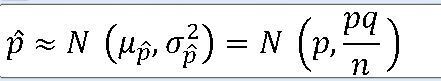


==> 두 모비율의 차 p_1 - p_2에 대한 90% 신뢰구간
x = np.arange(-5,5 , .001)

fig = plt.figure(figsize=(15,8))

ax = sns.lineplot(x , stats.norm.pdf(x, loc=0 , scale =1)) #정의역 범위 , 평균 = 0 , 표준편차 =1 인 정규분포 플롯

trust = 90#신뢰구간

# z_1 = round((0.05) / math.sqrt( 0.0018532 ) ,2)
# # z_2 = round((34.5 - 35) / math.sqrt(5.5**2 / 25) , 2)
z_1 = round(scipy.stats.norm.ppf(1 - (1-(trust/100))/2) ,3 )

ax.fill_between(x, stats.norm.pdf(x, loc=0 , scale =1) , 0 , where = (x<=z_1) & (x>=-z_1) , facecolor = 'skyblue') # x값 , y값 , 0 , x<=0 인곳 , 색깔


area = scipy.stats.norm.cdf(z_1) - scipy.stats.norm.cdf(-z_1)
plt.annotate('' , xy=(0, .1), xytext=(2 , .1)  , arrowprops = dict(facecolor = 'black'))

ax.vlines(x= z_1, ymin= 0 , ymax= stats.norm.pdf(z_1, loc=0 , scale =1) , color = 'black' , linestyle ='solid' , label ='{}'.format(2))
ax.vlines(x= -z_1, ymin= 0 , ymax= stats.norm.pdf(-z_1, loc=0 , scale =1) , color = 'black' , linestyle ='solid' , label ='{}'.format(2))

ax.text(2 , .1, f'P({-z_1}<=Z<={z_1}) : {round(area,4)}',fontsize=15)

ax.text(-5.5 , .25, f'신뢰구간 모평균에 대한 {trust}% : \n' + r'$\left(\widehat{p}_{1} - \widehat{p}_{2}\right)$' +f'-{z_1}' + r'$\sqrt{\dfrac{\widehat{p}_{1}\widehat{q}_{1}}{n}+\dfrac{\widehat{p}_{2}\widehat{q}_{2}}{m}}$' +' , '+ r'$\left(\widehat{p}_{1} - \widehat{p}_{2}\right)$' +f'+ {z_1}' + r'$\sqrt{\dfrac{\widehat{p}_{1}\widehat{q}_{1}}{n}+\dfrac{\widehat{p}_{2}\widehat{q}_{2}}{m}}$',fontsize=15)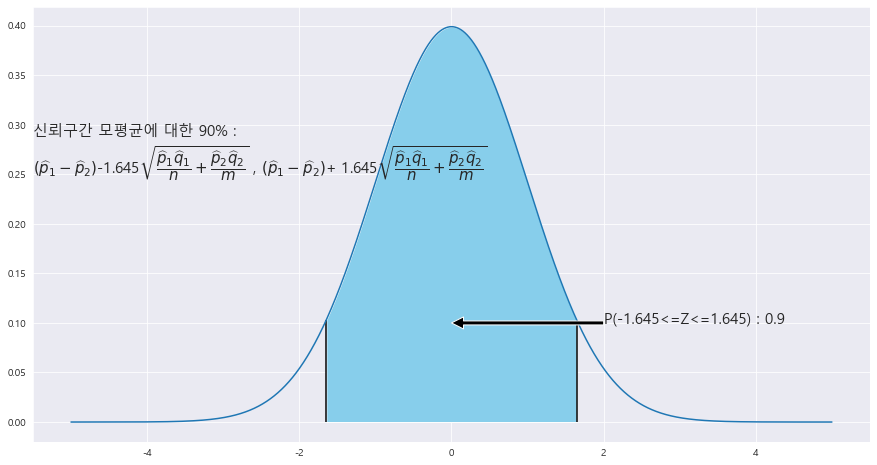
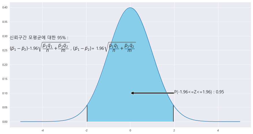
==> 두 모비율의 차 p_1 - p_2에 대한 95% 신뢰구간
x = np.arange(-5,5 , .001)

fig = plt.figure(figsize=(15,8))

ax = sns.lineplot(x , stats.norm.pdf(x, loc=0 , scale =1)) #정의역 범위 , 평균 = 0 , 표준편차 =1 인 정규분포 플롯

trust = 95#신뢰구간

# z_1 = round((0.05) / math.sqrt( 0.0018532 ) ,2)
# # z_2 = round((34.5 - 35) / math.sqrt(5.5**2 / 25) , 2)
z_1 = round(scipy.stats.norm.ppf(1 - (1-(trust/100))/2) ,3 )

ax.fill_between(x, stats.norm.pdf(x, loc=0 , scale =1) , 0 , where = (x<=z_1) & (x>=-z_1) , facecolor = 'skyblue') # x값 , y값 , 0 , x<=0 인곳 , 색깔


area = scipy.stats.norm.cdf(z_1) - scipy.stats.norm.cdf(-z_1)
plt.annotate('' , xy=(0, .1), xytext=(2 , .1)  , arrowprops = dict(facecolor = 'black'))

ax.vlines(x= z_1, ymin= 0 , ymax= stats.norm.pdf(z_1, loc=0 , scale =1) , color = 'black' , linestyle ='solid' , label ='{}'.format(2))
ax.vlines(x= -z_1, ymin= 0 , ymax= stats.norm.pdf(-z_1, loc=0 , scale =1) , color = 'black' , linestyle ='solid' , label ='{}'.format(2))

ax.text(2 , .1, f'P({-z_1}<=Z<={z_1}) : {round(area,4)}',fontsize=15)

ax.text(-5.5 , .25, f'신뢰구간 모평균에 대한 {trust}% : \n' + r'$\left(\widehat{p}_{1} - \widehat{p}_{2}\right)$' +f'-{z_1}' + r'$\sqrt{\dfrac{\widehat{p}_{1}\widehat{q}_{1}}{n}+\dfrac{\widehat{p}_{2}\widehat{q}_{2}}{m}}$' +' , '+ r'$\left(\widehat{p}_{1} - \widehat{p}_{2}\right)$' +f'+ {z_1}' + r'$\sqrt{\dfrac{\widehat{p}_{1}\widehat{q}_{1}}{n}+\dfrac{\widehat{p}_{2}\widehat{q}_{2}}{m}}$',fontsize=15)
==> 두 모비율의 차 p_1 - p_2에 대한 99% 신뢰구간
x = np.arange(-5,5 , .001)

fig = plt.figure(figsize=(15,8))

ax = sns.lineplot(x , stats.norm.pdf(x, loc=0 , scale =1)) #정의역 범위 , 평균 = 0 , 표준편차 =1 인 정규분포 플롯

trust = 99#신뢰구간

# z_1 = round((0.05) / math.sqrt( 0.0018532 ) ,2)
# # z_2 = round((34.5 - 35) / math.sqrt(5.5**2 / 25) , 2)
z_1 = round(scipy.stats.norm.ppf(1 - (1-(trust/100))/2) ,3 )

ax.fill_between(x, stats.norm.pdf(x, loc=0 , scale =1) , 0 , where = (x<=z_1) & (x>=-z_1) , facecolor = 'skyblue') # x값 , y값 , 0 , x<=0 인곳 , 색깔


area = scipy.stats.norm.cdf(z_1) - scipy.stats.norm.cdf(-z_1)
plt.annotate('' , xy=(0, .1), xytext=(2 , .1)  , arrowprops = dict(facecolor = 'black'))

ax.vlines(x= z_1, ymin= 0 , ymax= stats.norm.pdf(z_1, loc=0 , scale =1) , color = 'black' , linestyle ='solid' , label ='{}'.format(2))
ax.vlines(x= -z_1, ymin= 0 , ymax= stats.norm.pdf(-z_1, loc=0 , scale =1) , color = 'black' , linestyle ='solid' , label ='{}'.format(2))

ax.text(2 , .1, f'P({-z_1}<=Z<={z_1}) : {round(area,4)}',fontsize=15)

ax.text(-5.5 , .25, f'신뢰구간 모평균에 대한 {trust}% : \n' + r'$\left(\widehat{p}_{1} - \widehat{p}_{2}\right)$' +f'-{z_1}' + r'$\sqrt{\dfrac{\widehat{p}_{1}\widehat{q}_{1}}{n}+\dfrac{\widehat{p}_{2}\widehat{q}_{2}}{m}}$' +' , '+ r'$\left(\widehat{p}_{1} - \widehat{p}_{2}\right)$' +f'+ {z_1}' + r'$\sqrt{\dfrac{\widehat{p}_{1}\widehat{q}_{1}}{n}+\dfrac{\widehat{p}_{2}\widehat{q}_{2}}{m}}$',fontsize=15)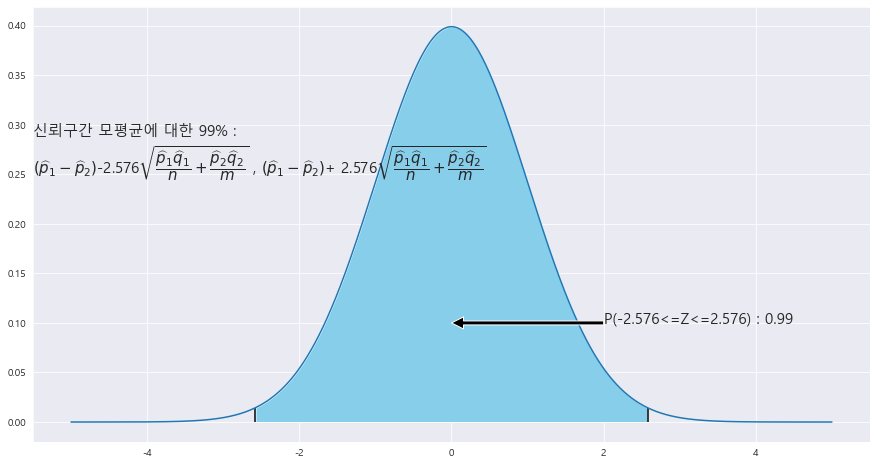
EX-01) 미혼 직장인 1089명 (남자 470명 , 여자 619명)을 대상으로 성인 전용 극장의 허용에 대해 설문 조사한 결과, 남성 254명과 여성 223명이 찬성하였다.
1> 남성과 여성의 성인 전용 극장의 허용에 대한 찬성률의 차이 p1 - p2를 추정
p1 = 254/470 =
p2 = 223/619
p1 - p2 = 0.1801
2> ^p1 - ^p2의 표준오차를 구하라.
^p1 - ^p2 ~ N(0.1801 , 0.5404 * (1-0.5404) / 470 + 0.3602 + (1-0.3602)/ 619 )
표준오차 = 루트(0.5404 * (1-0.5404) / 470 + 0.3602 + (1-0.3602)/ 619 ) = 0.03
3> | (^p1 -^p2) - (p1 - p2) | 에 대한 95% 오차 한계를 구하라.
x = np.arange(-5,5 , .001)

fig = plt.figure(figsize=(15,8))

ax = sns.lineplot(x , stats.norm.pdf(x, loc=0 , scale =1)) #정의역 범위 , 평균 = 0 , 표준편차 =1 인 정규분포 플롯

trust = 95#신뢰구간

# z_1 = round((0.05) / math.sqrt( 0.0018532 ) ,2)
# # z_2 = round((34.5 - 35) / math.sqrt(5.5**2 / 25) , 2)
z_1 = round(scipy.stats.norm.ppf(1 - (1-(trust/100))/2) ,3 )

ax.fill_between(x, stats.norm.pdf(x, loc=0 , scale =1) , 0 , where = (x<=z_1) & (x>=-z_1) , facecolor = 'skyblue') # x값 , y값 , 0 , x<=0 인곳 , 색깔


area = scipy.stats.norm.cdf(z_1) - scipy.stats.norm.cdf(-z_1)
plt.annotate('' , xy=(0, .1), xytext=(2 , .1)  , arrowprops = dict(facecolor = 'black'))

ax.vlines(x= z_1, ymin= 0 , ymax= stats.norm.pdf(z_1, loc=0 , scale =1) , color = 'black' , linestyle ='solid' , label ='{}'.format(2))
ax.vlines(x= -z_1, ymin= 0 , ymax= stats.norm.pdf(-z_1, loc=0 , scale =1) , color = 'black' , linestyle ='solid' , label ='{}'.format(2))

ax.text(2 , .1, f'P({-z_1}<=Z<={z_1}) : {round(area,4)}',fontsize=15)

ax.text(-5.5 , .25, f'신뢰구간 모평균에 대한 {trust}% : \n' + r'$\left(\widehat{p}_{1} - \widehat{p}_{2}\right)$' +f'-{z_1}' + r'$\sqrt{\dfrac{\widehat{p}_{1}\widehat{q}_{1}}{n}+\dfrac{\widehat{p}_{2}\widehat{q}_{2}}{m}}$' +' , '+ r'$\left(\widehat{p}_{1} - \widehat{p}_{2}\right)$' +f'+ {z_1}' + r'$\sqrt{\dfrac{\widehat{p}_{1}\widehat{q}_{1}}{n}+\dfrac{\widehat{p}_{2}\widehat{q}_{2}}{m}}$',fontsize=15)
p1 = 254/470
p2 = 223/619
A = 470
B = 619

ax.text(2 , .25, f'모비율의 차에 대한 신뢰구간 {trust}% : \n' + f'{round((p1-p2) - (z_1)*math.sqrt(p1*(1-p1)/A + p2*(1-p2)/B),3)} ~ {round((p1-p2) + (z_1)*math.sqrt(p1*(1-p1)/A + p2*(1-p2)/B),3)}' , fontsize= 15)

ax.text(1 , .35, f' 신뢰구간 {trust}% 에 대한 오차 한계( ' +r'$e_{%d}) : $ '% trust + f'\n' + r'${%.3f}\sqrt{\dfrac{\widehat{p}_{1}\widehat{q}_{1}}{n}+\dfrac{\widehat{p}_{2}\widehat{q}_{2}}{m}}$ = '% z_1 + f'{round((z_1)*math.sqrt(p1*(1-p1)/A + p2*(1-p2)/B),3)} ' , fontsize= 15)
==> r연산자로 string 받을 때 { } 중괄호 안에 %연산자를 집어넣어주는것 기억하기!!!
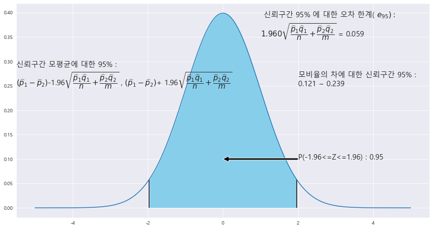
4> p_1 - p_2 에 대한 95% 신뢰구간을 구하라.
(0.121 ~ 0.239)
EX-02) 두 종류의 약품 A, B의 효능을 조사하기 위하여 동일한 조건을 가진 환자 400명 중 250명은 약품 A로 치료하고, 다른 150명은 약품 B로 치료한 결과 , 각각 215명과 124명이 효과를 얻었다. 두 약품의 효율의 차이에 대한 90% 신뢰구간을 구하라.
N = 250
M = 150
p_1 = 215/250
p_2 = 124/150
(-0.029 , 0.096)
x = np.arange(-5,5 , .001)

fig = plt.figure(figsize=(15,8))

ax = sns.lineplot(x , stats.norm.pdf(x, loc=0 , scale =1)) #정의역 범위 , 평균 = 0 , 표준편차 =1 인 정규분포 플롯

trust = 90#신뢰구간

# z_1 = round((0.05) / math.sqrt( 0.0018532 ) ,2)
# # z_2 = round((34.5 - 35) / math.sqrt(5.5**2 / 25) , 2)
z_1 = round(scipy.stats.norm.ppf(1 - (1-(trust/100))/2) ,3 )

ax.fill_between(x, stats.norm.pdf(x, loc=0 , scale =1) , 0 , where = (x<=z_1) & (x>=-z_1) , facecolor = 'skyblue') # x값 , y값 , 0 , x<=0 인곳 , 색깔


area = scipy.stats.norm.cdf(z_1) - scipy.stats.norm.cdf(-z_1)
plt.annotate('' , xy=(0, .1), xytext=(2 , .1)  , arrowprops = dict(facecolor = 'black'))

ax.vlines(x= z_1, ymin= 0 , ymax= stats.norm.pdf(z_1, loc=0 , scale =1) , color = 'black' , linestyle ='solid' , label ='{}'.format(2))
ax.vlines(x= -z_1, ymin= 0 , ymax= stats.norm.pdf(-z_1, loc=0 , scale =1) , color = 'black' , linestyle ='solid' , label ='{}'.format(2))

ax.text(2 , .1, f'P({-z_1}<=Z<={z_1}) : {round(area,4)}',fontsize=15)

ax.text(-5.5 , .25, f'신뢰구간 모평균에 대한 {trust}% : \n' + r'$\left(\widehat{p}_{1} - \widehat{p}_{2}\right)$' +f'-{z_1}' + r'$\sqrt{\dfrac{\widehat{p}_{1}\widehat{q}_{1}}{n}+\dfrac{\widehat{p}_{2}\widehat{q}_{2}}{m}}$' +' , '+ r'$\left(\widehat{p}_{1} - \widehat{p}_{2}\right)$' +f'+ {z_1}' + r'$\sqrt{\dfrac{\widehat{p}_{1}\widehat{q}_{1}}{n}+\dfrac{\widehat{p}_{2}\widehat{q}_{2}}{m}}$',fontsize=15)
p1 = 215/250
p2 = 124/150
A = 250
B = 150

ax.text(2 , .25, f'모비율의 차에 대한 신뢰구간 {trust}% : \n' + f'{round((p1-p2) - (z_1)*math.sqrt(p1*(1-p1)/A + p2*(1-p2)/B),3)} ~ {round((p1-p2) + (z_1)*math.sqrt(p1*(1-p1)/A + p2*(1-p2)/B),3)}' , fontsize= 15)

ax.text(1 , .35, f' 신뢰구간 {trust}% 에 대한 오차 한계( ' +r'$e_{%d}) : $ '% trust + f'\n' + r'${%.3f}\sqrt{\dfrac{\widehat{p}_{1}\widehat{q}_{1}}{n}+\dfrac{\widehat{p}_{2}\widehat{q}_{2}}{m}}$ = '% z_1 + f'{round((z_1)*math.sqrt(p1*(1-p1)/A + p2*(1-p2)/B),3)} ' , fontsize= 15)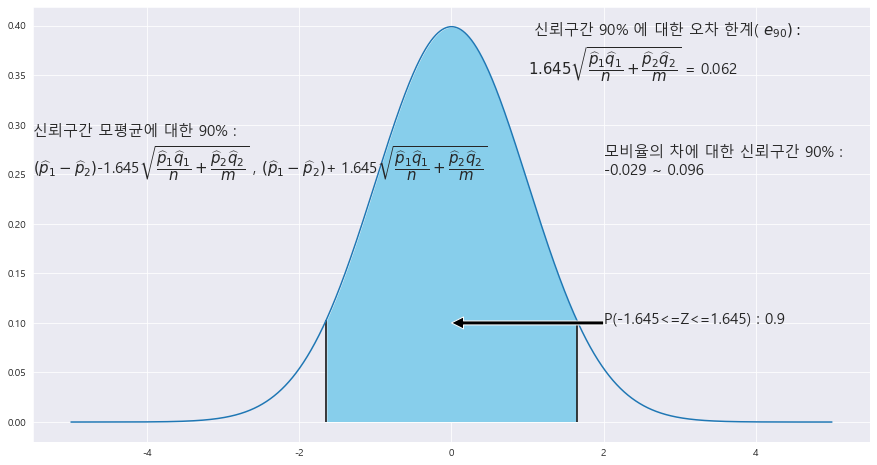
출처 : [쉽게 배우는 생활속의 통계학] [북스힐 , 이재원]
※혼자 공부 정리용
'기초통계 > 대표본 추정' 카테고리의 다른 글
| ★모비율,모평균에 대한 오차한계★오차한계(신뢰구간의 절반)★기초통계학-[연습문제 -07] (0) | 2023.01.12 |
|---|---|
| ★모평균의 차에 대한 신뢰구간★모비율에 대한 표본크기 구하기★표본의 크기★기초통계학-[대표본 추정 -06] (0) | 2023.01.12 |
| ★모평균 차의 구간추정★기초통계학-[대표본 추정 -05] (0) | 2023.01.11 |
| ★모비율의 신뢰구간★기초통계학-[대표본 추정 -04] (0) | 2023.01.11 |
| ★신뢰구간★신뢰도★구간추정★기초통계학-[대표본 추정 -03] (0) | 2023.01.11 |