sympy.solve() 방정식 값구하기★정규분포의 Z값 궁금할땐 ppf 사용!!!★삼각형그리드★평균,분산구하기★연속확률변수★기초통계학-[Chapter06 - 연습문제-11]

10. 확률변수 X의 확률밀도함수가 다음과 같을 때, P(X<=a)=1/4인 상수 a를 구하라. ==> 연속확률변수

 

f(x) = 2x , 0<=x<=1

0 , otherwise

from sympy import Integral,  Symbol , pprint ,solve

x = Symbol('x')
f = 2 * x

f_x_m = f *x

pprint(Integral(f_x_m, x).doit()) #이쁘게 출력
print('===')

mean_x = Integral(f_x_m, (x, (0, 1))).doit()
print("평균 : {}".format(mean_x)) #적분변수 , 아래끝 , 위끝

var_x = Integral(f_x_m *x, (x, (0, 1))).doit() - math.pow(mean_x , 2)

print("분산 : {}".format(var_x))

==> Symbol 과 Integral , solve 라이브러리 불러온다!

 

https://knowallworld.tistory.com/261

균등분포,F-분포 헷갈림★PDF,PPF,CDF★표준정규확률 구할땐 CDF★기초통계학-[Chapter06 - 연습문제-09]

 

균등분포,F-분포 헷갈림★PDF,PPF,CDF★표준정규확률 구할땐 CDF★기초통계학-[Chapter06 - 연습문제-09]

==> mean = 인테그랄(범위) x*f(X)

==> var = 인테그랄(범위) x**2*f(x)  - 평균의 제곱

#P(X<=a) = P(Z<= (a-평균)/표준편차)) = 1/4
#(a-평균)/표준편차) = X_r
X_r = scipy.stats.norm.ppf(0.25)
print(X_r)
print(var_x)
print(math.sqrt(var_x))
equation = (x- mean_x) / math.sqrt(var_x) - X_r
d = solve(equation)
print(d)

P(X<=a) = 0.25 = P(Z<= (a-평균)/(표준편차) ) 

==> scipy.stats.norm.ppf(0.25) ==> Z값 구할 수 있다!!

==> Z = -0.6744897501960817

 

==> sympy의 solve 함수 불러온다!!!! ==> 옆에 값이 0이어만 계산이 가능하다.

 

==> (x- mean_x) / math.sqrt(var_x) - X_r = 

 

a = 0.507687907931844

 

11. 연속확률변수 X의 확률밀도함수 f(x)가 x축범위가 (0,1) 인 이등변삼각형일 때

import matplotlib.tri as mtri

fig = plt.figure(figsize=(15,8))
x = np.array([0,1,2]) #삼각형의 x좌표
y = np.array([0,1 , 0]) #삼각형의 y좌표

triangles = [[0,1,2]] #삼각형의 점 개수
triang = mtri.Triangulation(x,y , triangles)

plt.title("삼각 그리드")
plt.triplot(triang , 'ko-')
plt.fill_between(x , x , 0 , where = (x<= 1) & (x>=0) , color = 'orange')
plt.fill_between(x , -x+2 , 0 , where =  (x>=1) & (x<= 2) )

plt.xlim(-0.1 , 2.1)
plt.ylim(-0.1 , 1.6)

plt.text(0.5 , 0.6 , 'y = x' , fontsize = 13 , rotation = 33)
plt.text(1.5 , 0.5 , 'y = -x+2' , fontsize = 13 , rotation = -33)
plt.show()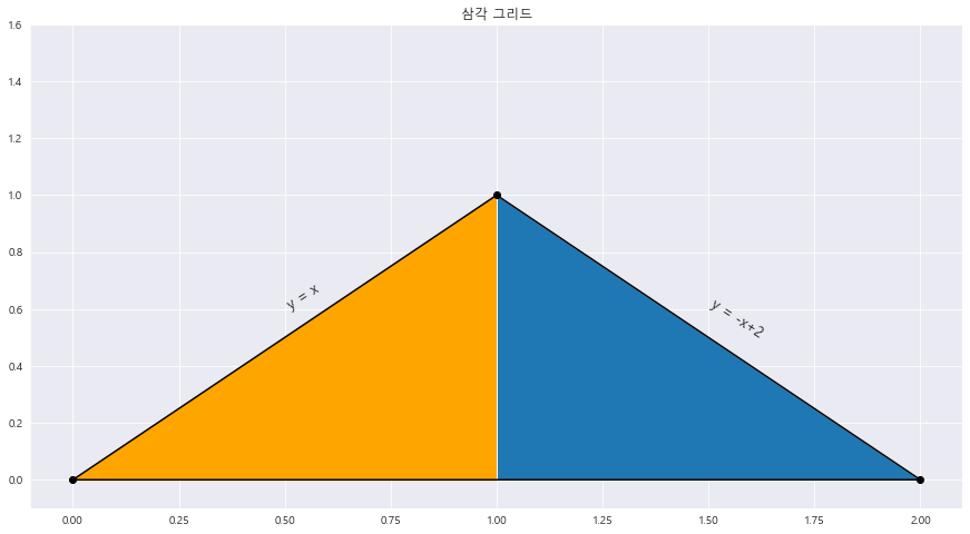

삼각그리드

 

 

==> 삼각그리드 그리기

 

1> 상수 k값 구하기

k = sympy.Symbol('k')
sol_k = 2*k*(1/2) -1 # k * 2 * 1/2
k_sol = solve(sol_k)
print(k_sol)

k =1

 

 

2> P(X<=0.6) = 0.6 * (0.6) /2 = 0.18

from sympy import Integral,  Symbol , pprint ,solve

x = Symbol('x')
f_1 =  x
f_2 = -x +2
f_x_1_m = f_1 *x
f_x_2_m = f_2 *x

mean_x = Integral(f_x_1_m, (x, (0, 1))).doit() + Integral(f_x_2_m, (x, (1, 2))).doit()
print("평균 : {}".format(mean_x)) #적분변수 , 아래끝 , 위끝

var_x = Integral(f_x_1_m*x, (x, (0, 1))).doit() + Integral(f_x_2_m*x, (x, (1, 2))).doit() - math.pow(mean_x, 2)

print("분산 : {}".format(var_x)) #적분변수 , 아래끝 , 위끝

평균 : 1
분산 : 0.166666666666667

x_0_6 = round((0.6-(mean_x)) / math.sqrt(var_x),8)
x_0 = round( (0-mean_x) / math.sqrt(var_x) , 4)
print(x_0_6)
print(x_0)
print(scipy.stats.norm.cdf(-0.97979590))

-0.97979590
-2.4495
0.16359343818253824

 

==> 오차발생 추후 생각해보자

 

3> P(0.5<=X<=1.5) = (1-0.5) * 0.5 / 2 * 2 + (1 * 0.5) = 0.25 + 0.5 = 0.75

 

x_0_1_5 = round((1.5-(mean_x)) / math.sqrt(var_x),8)
x_0_5 = round( (0.5-mean_x) / math.sqrt(var_x) , 4)
print(x_0_1_5)
print(x_0_5)
print(scipy.stats.norm.cdf(1.2247) - scipy.stats.norm.cdf(-1.2247) )

1.22474487
-1.2247
0.7793117258581086

P(X <=1.5) - P(X<=0.5) = 0.7793 ==> 오차발생

 

 

4> P(1.2<= X<=2) =(2-1.2) * 0.8 / 2 = 0.8 * 0.8 / 2 = 0.32

 

x_0_2 = round((2-(mean_x)) / math.sqrt(var_x),8)
x_0_1_2 = round( (1.2-mean_x) / math.sqrt(var_x) , 4)
print(x_0_2)
print(x_0_1_2)
print(scipy.stats.norm.cdf(2.4494) - scipy.stats.norm.cdf(0.4899) )

P(1.2<= X<=2) = P(X<=2) - P(X<=1.2) =  0.3049 ==> 오차발생

 

 

12. 확률밀도함수에 대한 확률 구하기

a_x= np.arange(0,20,.1) # len(a_x) = 20

a_y = np.full((1,len(a_x)) , 0.02) #1행 20열값을 0.02로 가득채워라
print(a_y)

A = pd.DataFrame([a_x , *a_y])
A= A.T
a_x= np.arange(20,30,.1) # len(a_x) = 20

a_y = np.full((1,len(a_x)) , 0.04) #1행 20열값을 0.02로 가득채워라

B= pd.DataFrame([a_x , *a_y])
B = B.T

a_x= np.arange(30,41,.1) # len(a_x) = 20

a_y = np.full((1,len(a_x)) , 0.02) #1행 20열값을 0.02로 가득채워라

C= pd.DataFrame([a_x , *a_y])
C = C.T

A = pd.concat([A,B,C]).reset_index()
A = A.iloc[ : , 1:]
A

 

 

1> P(X>=35) = 0.1

 

fig = plt.figure(figsize=(15,8))

# ax = sns.distplot(x = A[0] , y=A[1])
ax= sns.lineplot(x= A[0] , y= A[1])
ax.set_xlim(-1 , 45)
ax.set_ylim(0 , 0.05)
ax.set_xlabel('경기에참여하는 시간' , fontsize = 12)
ax.set_ylabel('확률밀도함수 f(x)' , fontsize= 12 , rotation=0 , labelpad = 20)


ax.fill_between(A[0] , A[1] , 0 , where =  (A[0]>=35))

area = (40-35) * 0.02
ax.text(29 , 0.015 , 'P(X>=35) = {}'.format(area) , fontsize= 13)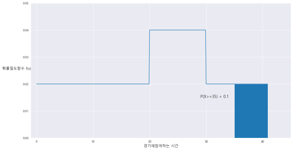

연속확률분포_1

2> P(X<=25) = 0.6

fig = plt.figure(figsize=(15,8))

# ax = sns.distplot(x = A[0] , y=A[1])
ax= sns.lineplot(x= A[0] , y= A[1])
ax.set_xlim(-1 , 45)
ax.set_ylim(0 , 0.05)
ax.set_xlabel('경기에참여하는 시간' , fontsize = 12)
ax.set_ylabel('확률밀도함수 f(x)' , fontsize= 12 , rotation=0 , labelpad = 20)


ax.fill_between(A[0] , A[1] , 0 , where =  (A[0]<=25))

area = (25-20) * 0.04 + (20*0.02)
ax.text(26 , 0.015 , 'P(X<=25) = {}'.format(round(area,2)) , fontsize= 13)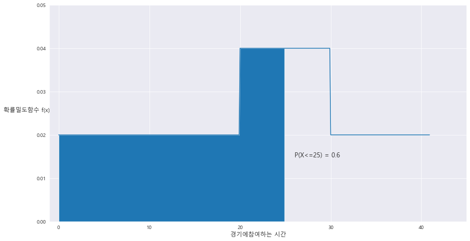

3> P(15<=X<=35) = 0.6

fig = plt.figure(figsize=(15,8))

# ax = sns.distplot(x = A[0] , y=A[1])
ax= sns.lineplot(x= A[0] , y= A[1])
ax.set_xlim(-1 , 45)
ax.set_ylim(0 , 0.05)
ax.set_xlabel('경기에참여하는 시간' , fontsize = 12)
ax.set_ylabel('확률밀도함수 f(x)' , fontsize= 12 , rotation=0 , labelpad = 20)


ax.fill_between(A[0] , A[1] , 0 , where =  (A[0]<=35) & (A[0]>=15))

area = (30-20) * 0.04 + ((35-30)*0.02) + ((20-15) *0.02)
ax.text(8 , 0.015 , 'P(15<=X<=35) = {}'.format(round(area,2)) , fontsize= 13)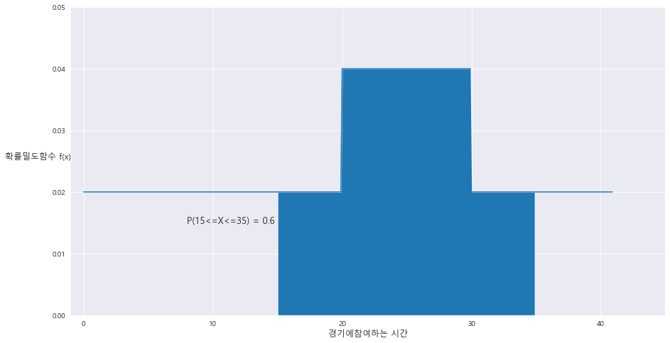

연속확률분포_3

출처 :  [쉽게 배우는 생활속의 통계학]  [북스힐 , 이재원] 

※혼자 공부 정리용