stats.norm.cdf()★표준정규분포 넓이 구하기!!★ax.lineplot★정규분포(Normal Distribution)★기초통계학-[Chapter06 - 연속확률분포-02]

1. 정규분포(Normal Distribution)

 

==> 자료 집단에 대한 도수히스토그램은 자료의 수가 많을 수록 종 모양에 가까운 형태로 나타난다.

 

==> 종 모양의 확률분포를 정규분포라고 한다.

 

 

1>정규분포의 성질

 

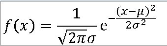
평균 myu(뮤)와 분산에 대하여 확률밀도함수를 가지는 연속확률분포

 

https://knowallworld.tistory.com/216

★distplot , histplot , twinx(), ticker , axvline()★정규분포 그래프★기초통계학-[Chapter03 - 05]

 

정규분포

정규분포 식

==> 정규분포는 중심위치에서 꼭짓점이 하나인 종 모양이다. 평균, 중위수, 최빈값이 분포의 중심위치로 동일하다.

 

==> 평균은 서로 다르지만, 표준편차가 동일한 경우 중심 위치는 다르지만 모양은 동일하게 나타난다.

 

==> 평균은 동일하지만 , 표준편차가 다른 경우 자료가 평균에 밀집하고 클수록 자료가 퍼지는 모양을 갖는다.

 

x = np.arange(-10,10 ,.001)
fig  = plt.figure(figsize= (15,8))
ax = sns.lineplot(x , stats.norm.pdf(x, loc=0 , scale =1)) #정의역 범위 , 평균 = 0 , 표준편차 =2 인 정규분포 플롯
sns.lineplot(x , stats.norm.pdf(x, loc=8 , scale =1)) #정의역 범위 , 평균 = 0 , 표준편차 =2 인 정규분포 플롯
sns.lineplot(x , stats.norm.pdf(x, loc=0 , scale= 2)) #정의역 범위 , 평균 = 0 , 표준편차 =2 인 정규분포 플롯
sns.lineplot(x , stats.norm.pdf(x, loc=0 , scale =5)) #정의역 범위 , 평균 = 0 , 표준편차 =5 인 정규분포 플롯
ax.axvline(x= 0, ymin=0 , ymax=1 , color = 'black' , linestyle ='solid' , label ='{}'.format(2))
ax.text(0, .41, f'평균 : {round(0,2)}',fontsize=13)
plt.legend(['N(0,1)' , 'N(2,1)' , 'N(0,2)' , 'N(0,5)'] , fontsize = 15)

정규분포

2. 표준정규분포(Standard Normal Distribution)

 

==> 평균이 0이고 , 분산이 1 인 정규분포

 

표준정규분포

표준정규분포의 확률밀도함수

x = np.arange(-5,5 , .001)

fig = plt.figure(figsize=(15,8))

ax = sns.lineplot(x , stats.norm.pdf(x, loc=0 , scale =1)) #정의역 범위 , 평균 = 0 , 표준편차 =2 인 정규분포 플롯
ax.fill_between(x, stats.norm.pdf(x, loc=0 , scale =1) , 0 , where = x>=0 , facecolor = 'red')

ax.fill_between(x, stats.norm.pdf(x, loc=0 , scale =1) , 0 , where = x<=0 , facecolor = 'blue') # x값 , y값 , 0 , x<=0 인곳 , 색깔


ax.text(0.3, .10, f'P(Z>=0)  \n{0.5}',fontsize=20)
ax.text(-1, .10, f'P(Z<0)  \n{0.5}',fontsize=20)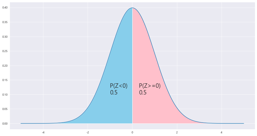

==> 확률 P(Z<=0) = P(Z>=0)

 

 

꼬리확률(Tail Probability)

 

==> P(Z<=a) = P(Z>=a)

 

 

x = np.arange(-5,5 , .001)

fig = plt.figure(figsize=(15,8))

ax = sns.lineplot(x , stats.norm.pdf(x, loc=0 , scale =1)) #정의역 범위 , 평균 = 0 , 표준편차 =2 인 정규분포 플롯


ax.fill_between(x, stats.norm.pdf(x, loc=0 , scale =1) , 0 , where = (-3<x) & (x<3) , facecolor = 'skyblue') #where 절 and는 &활용
ax.vlines(x= 3, ymin= 0 , ymax= stats.norm.pdf(3, loc=0 , scale =1) + 0.1 , color = 'black' , linestyle ='solid' , label ='{}'.format(2))
ax.vlines(x= -3, ymin= 0 , ymax= stats.norm.pdf(-3, loc=0 , scale =1) + 0.1 , color = 'black' , linestyle ='solid' , label ='{}'.format(2))
plt.annotate('' , xy=(-3, .10), xytext=(0 , .10)  , arrowprops = dict(facecolor = 'black'))
plt.annotate('' , xy=(3, .10), xytext=(0 , .10)  , arrowprops = dict(facecolor = 'black'))
ax.text(-1, .12, f'P(-3<=Z<=3) : {0.997}',fontsize=15)




ax.fill_between(x, stats.norm.pdf(x, loc=0 , scale =1) , 0 , where = (-2<x) & (x<2) , facecolor = 'skyblue') #where 절 and는 &활용
ax.vlines(x= 2, ymin= 0 , ymax= stats.norm.pdf(2, loc=0 , scale =1) + 0.2 , color = 'green' , linestyle ='solid' , label ='{}'.format(2))
ax.vlines(x= -2, ymin= 0 , ymax= stats.norm.pdf(-2, loc=0 , scale =1) + 0.2 , color = 'green' , linestyle ='solid' , label ='{}'.format(2))
plt.annotate('' , xy=(-2, .20), xytext=(0 , .20)  , arrowprops = dict(facecolor = 'black'))
plt.annotate('' , xy=(2, .20), xytext=(0 , .20)  , arrowprops = dict(facecolor = 'black'))
ax.text(-1, .22, f'P(-2<=Z<=2) : {0.954}',fontsize=15)






ax.fill_between(x, stats.norm.pdf(x, loc=0 , scale =1) , 0 , where = (-1<x) & (x<1) , facecolor = 'pink') #where 절 and는 &활용
ax.vlines(x= 1, ymin= 0 , ymax= stats.norm.pdf(1, loc=0 , scale =1) + 0.3 , color = 'blue' , linestyle ='solid' , label ='{}'.format(2))
ax.vlines(x= -1, ymin= 0 , ymax= stats.norm.pdf(-1, loc=0 , scale =1) + 0.3 , color = 'blue' , linestyle ='solid' , label ='{}'.format(2))
plt.annotate('' , xy=(-1, .50), xytext=(0 , .50)  , arrowprops = dict(facecolor = 'black'))
plt.annotate('' , xy=(1, .50), xytext=(0 , .50)  , arrowprops = dict(facecolor = 'black'))
ax.text(-1, .52, f'P(-1<=Z<=1) : {0.683}',fontsize=15)

표준정규분포

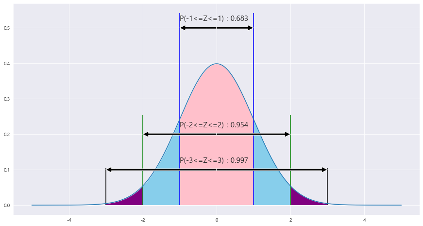
==> 경험적 규칙에 따라

 

==> P(|Z| <=1) = 0.683 , P(|Z| <=2) = 0.954 , P(|Z| <=1) = 0.997

 

 

 

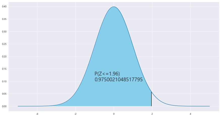
EX-01) P(Z<= 1.96) 

 

x = np.arange(-5,5 , .001)

fig = plt.figure(figsize=(15,8))

ax = sns.lineplot(x , stats.norm.pdf(x, loc=0 , scale =1)) #정의역 범위 , 평균 = 0 , 표준편차 =2 인 정규분포 플롯
#ax.fill_between(x, stats.norm.pdf(x, loc=0 , scale =1) , 0 , where = x>=0  , facecolor = 'pink')

ax.fill_between(x, stats.norm.pdf(x, loc=0 , scale =1) , 0 , where = x<=1.96 , facecolor = 'skyblue') # x값 , y값 , 0 , x<=0 인곳 , 색깔


#ax.text(0.3, .10, f'P(Z>=0)  \n{0.5}',fontsize=20)
area = stats.norm(0,1).cdf(1.96) # area 계산!!
ax.text(-1, .10, f'P(Z<=1.96)  \n{area}',fontsize=20)
ax.vlines(x= 1.96, ymin= 0 , ymax= stats.norm.pdf(1.96, loc=0 , scale =1) , color = 'black' , linestyle ='solid' , label ='{}'.format(2))

 

표준정규분포 넓이

 

EX-02) P(Z>= 2.03)

 

x = np.arange(-5,5 , .001)

fig = plt.figure(figsize=(15,8))

ax = sns.lineplot(x , stats.norm.pdf(x, loc=0 , scale =1)) #정의역 범위 , 평균 = 0 , 표준편차 =2 인 정규분포 플롯
#ax.fill_between(x, stats.norm.pdf(x, loc=0 , scale =1) , 0 , where = x>=0  , facecolor = 'pink')

ax.fill_between(x, stats.norm.pdf(x, loc=0 , scale =1) , 0 , where = x>=2.03 , facecolor = 'skyblue') # x값 , y값 , 0 , x<=0 인곳 , 색깔


#ax.text(0.3, .10, f'P(Z>=0)  \n{0.5}',fontsize=20)
area = 1- stats.norm.cdf(2.03) #넓이 구하기!!!!!
ax.text(2.5 , .05, f'P(Z>=2.03) : {round(area,4)}',fontsize=15)
plt.annotate('' , xy=(2.2, .02), xytext=(2.5 , .04)  , arrowprops = dict(facecolor = 'black'))
ax.vlines(x= 2.03, ymin= 0 , ymax= stats.norm.pdf(2.03, loc=0 , scale =1) , color = 'black' , linestyle ='solid' , label ='{}'.format(2))

표준정규분포 넓이 구하기

EX-03) P(Z<= -0.57)

 

x = np.arange(-5,5 , .001)

fig = plt.figure(figsize=(15,8))

ax = sns.lineplot(x , stats.norm.pdf(x, loc=0 , scale =1)) #정의역 범위 , 평균 = 0 , 표준편차 =2 인 정규분포 플롯
#ax.fill_between(x, stats.norm.pdf(x, loc=0 , scale =1) , 0 , where = x>=0  , facecolor = 'pink')

ax.fill_between(x, stats.norm.pdf(x, loc=0 , scale =1) , 0 , where = x<=-0.57 , facecolor = 'skyblue') # x값 , y값 , 0 , x<=0 인곳 , 색깔


#ax.text(0.3, .10, f'P(Z>=0)  \n{0.5}',fontsize=20)
area =  stats.norm.cdf(-0.57)
ax.text(-3 , .11, f'P(Z<=-0.57) : {round(area,4)}',fontsize=15)
plt.annotate('' , xy=(-1.7, .02), xytext=(-2 , .1)  , arrowprops = dict(facecolor = 'black'))
ax.vlines(x= -0.57, ymin= 0 , ymax= stats.norm.pdf(-0.57, loc=0 , scale =1) , color = 'black' , linestyle ='solid' , label ='{}'.format(2))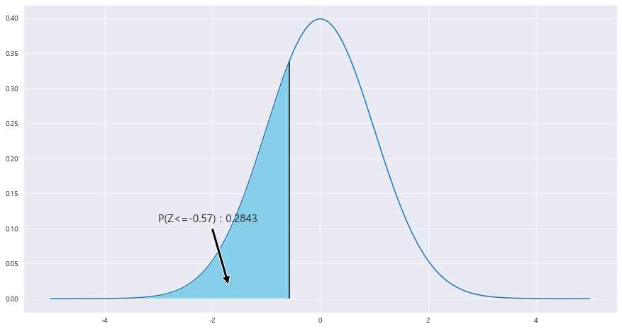

표준정규분포

EX-04) P(-1.75<=Z<= 2.12)

 

= P(Z<=2.12) - P(Z<=-1.75) 

 

x = np.arange(-5,5 , .001)

fig = plt.figure(figsize=(15,8))

ax = sns.lineplot(x , stats.norm.pdf(x, loc=0 , scale =1)) #정의역 범위 , 평균 = 0 , 표준편차 =2 인 정규분포 플롯
#ax.fill_between(x, stats.norm.pdf(x, loc=0 , scale =1) , 0 , where = x>=0  , facecolor = 'pink')

ax.fill_between(x, stats.norm.pdf(x, loc=0 , scale =1) , 0 , where = (x<=2.12) & (x>=-1.75) , facecolor = 'skyblue') # x값 , y값 , 0 , x<=0 인곳 , 색깔


#ax.text(0.3, .10, f'P(Z>=0)  \n{0.5}',fontsize=20)
area =  stats.norm.cdf(2.12) - stats.norm.cdf(-1.75)
ax.text(-3 , .17, f'P(-1.75<=Z<=2.12 : {round(area,4)}',fontsize=15)
plt.annotate('' , xy=(0, .15), xytext=(-2 , .15)  , arrowprops = dict(facecolor = 'black'))
ax.vlines(x= 2.12, ymin= 0 , ymax= stats.norm.pdf(-2.12, loc=0 , scale =1) , color = 'black' , linestyle ='solid' , label ='{}'.format(2))
ax.vlines(x= -1.75, ymin= 0 , ymax= stats.norm.pdf(-1.75, loc=0 , scale =1) , color = 'black' , linestyle ='solid' , label ='{}'.format(2))

P(-1.75 <= Z <= 2.12)

EX-05) P(-1.03<=Z<= 1.03)

 

= P(0<=Z<=1.03) * 2 = ( P(Z<=1.03) - P(Z<=0) ) * 2 = 

 

x = np.arange(-5,5 , .001)

fig = plt.figure(figsize=(15,8))

ax = sns.lineplot(x , stats.norm.pdf(x, loc=0 , scale =1)) #정의역 범위 , 평균 = 0 , 표준편차 =2 인 정규분포 플롯
#ax.fill_between(x, stats.norm.pdf(x, loc=0 , scale =1) , 0 , where = x>=0  , facecolor = 'pink')

ax.fill_between(x, stats.norm.pdf(x, loc=0 , scale =1) , 0 , where = (x<=1.03) & (x>=-1.03) , facecolor = 'skyblue') # x값 , y값 , 0 , x<=0 인곳 , 색깔


#ax.text(0.3, .10, f'P(Z>=0)  \n{0.5}',fontsize=20)
area =  ( stats.norm.cdf(1.03) - stats.norm.cdf(0) ) * 2
ax.text(-3 , .27, f'P(-1.03<=Z<=1.03 : {round(area,4)}',fontsize=15)
plt.annotate('' , xy=(0, .25), xytext=(-2 , .25)  , arrowprops = dict(facecolor = 'black'))
ax.vlines(x= 1.03, ymin= 0 , ymax= stats.norm.pdf(-1.03, loc=0 , scale =1) , color = 'black' , linestyle ='solid' , label ='{}'.format(2))
ax.vlines(x= -1.03, ymin= 0 , ymax= stats.norm.pdf(-1.03, loc=0 , scale =1) , color = 'black' , linestyle ='solid' , label ='{}'.format(2))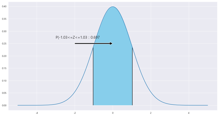

P(-1.03 <= Z <= 1.03)

출처 :  [쉽게 배우는 생활속의 통계학]  [북스힐 , 이재원] 

※혼자 공부 정리용